Principal components analysis (PCA) is a statistical technique that allows identifying underlying linear patterns in a
data set so it can be expressed in terms of another data set of a significantly lower dimension without much loss of information.
The final data set should explain most of the variance of the original data set by reducing the number of variables. The final variables will be named as principal components.
To illustrate the whole process, we will use the following data set, with only 2 dimensions.
| Instance | x1 | x2 | Instance | x1 | x2 | |
|---|---|---|---|---|---|---|
| 1 | 0.3 | 0.5 | 11 | 0.6 | 0.8 | |
| 2 | 0.4 | 0.3 | 12 | 0.4 | 0.6 | |
| 3 | 0.7 | 0.4 | 13 | 0.3 | 0.4 | |
| 4 | 0.5 | 0.7 | 14 | 0.6 | 0.5 | |
| 5 | 0.3 | 0.2 | 15 | 0.8 | 0.5 | |
| 6 | 0.9 | 0.8 | 16 | 0.8 | 0.9 | |
| 7 | 0.1 | 0.2 | 17 | 0.2 | 0.3 | |
| 8 | 0.2 | 0.5 | 18 | 0.7 | 0.7 | |
| 9 | 0.6 | 0.9 | 19 | 0.5 | 0.5 | |
| 10 | 0.2 | 0.2 | 20 | 0.6 | 0.4 |
The next scatter chart shows the values of the variable x2 against the values of the variable x1.

The objective is to convert that data set into a new one of only 1 dimension with minimal information loss.
The steps to perform principal components analysis are the following:
1. Subtract mean
The first step in the principal component analysis is to subtract the mean for each variable of the data set.
The next scatter chart shows how the data is rearranged in our example.
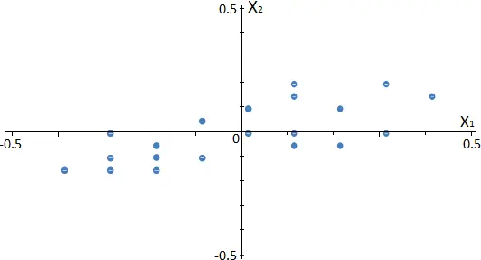
As shown, the subtraction of the mean results in a data translation, which has zero mean.
2. Calculate the covariance matrix
The covariance of two random variables measures the degree of variation from their means for each other.
The sign of the covariance provides us with information about the relation between them:
- If the covariance is positive, then the two variables increase and decrease together.
- If the covariance is negative, then when one variable increases, the other decreases, and vice versa.
These values determine the linear dependencies between the variables, which will be used to reduce the data set’s dimension.
Back to our example, the covariance matrix is shown next.
| x1 | x2 | |
|---|---|---|
| x1 | 0.33 | 0.25 |
| x2 | 0.25 | 0.41 |
The variance measures how the data is spread from the mean.
The diagonal values show the covariance of each variable and itself, and they equal their variance.
The off-diagonal values show the covariance between the two variables. In this case, these values are positive, which means that both variables increase and decrease together.
3. Calculate eigenvectors and eigenvalues
Eigenvectors are defined as those vectors whose directions remain unchanged after any linear transformation has been applied.
However, their length could not remain the same after the transformation, i.e., the result of this transformation is the vector multiplied by a scalar. This scalar is called eigenvalue, and each eigenvector has one associated with it.
The number of eigenvectors or components that we can calculate for each data set is equal to the data set’s dimension. In this case, we have a 2-dimensional data set, so the number of eigenvectors will be 2. The next image represents the eigenvectors for our example.
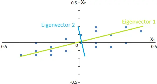
Since they are calculated from the covariance matrix described before, eigenvectors represent the directions in which the data have a higher variance. On the other hand, their respective eigenvalues determine the data set’s variance in that direction.
Once we have obtained these new directions, we can plot the data in terms of them, as shown in the following image for our example.
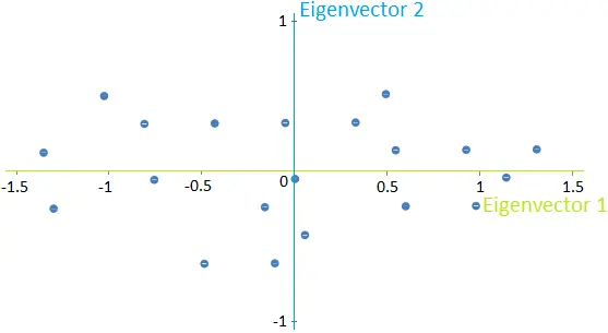
Note that the data has not changed; we are rewriting them in terms of these new directions instead of the previous x1-x2 directions.
4. Select principal components
Among the available eigenvectors that were previously calculated, we must select those onto which we project the data.
The selected eigenvectors will be called principal components.
To establish a criterion to select the eigenvectors, we must first define the relative variance of each and the total variance of a data set. The relative variance of an eigenvector measures how much information can be attributed to it. The total variance of a data set is the sum of the variance of all the variables.
These two concepts are determined by the eigenvalues. For our example, the following table shows the relative and cumulative variance for each eigenvector.
| Relative variance | Cumulative variance | |
|---|---|---|
| PC1 | 84.60 | 84.60 |
| PC2 | 15.40 | 100 |
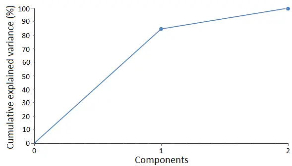
As we can see, the first eigenvector can explain almost 85% of all the data’s variance, while the second eigenvector explains around 15% of it. The following graph shows the cumulative variance for the components.
A common way to select the variables is to establish the amount of information that we want the final data set to explain.
If this amount of information decreases, the number of principal components that we select will decrease.
In this case, as we want to reduce the 2-dimensional data set into a 1-dimensional data set, we will select the first eigenvector as the principal component.
Consequently, the final reduced data set will explain 85% of the variance of the original one.
5. Reduce data dimension
Once we have selected the principal components, the data must be projected onto them. The following image shows the result of this projection for our example.

Although this projection can explain most of the variance of the original data, we have lost the information about the variance along with the second component. In general, this process is irreversible, which means that we cannot recover the original data from the projection.
Conclusions
Principal components analysis is a technique that allows us to identify the underlying dependencies of a data set and to reduce its dimensionality significantly attending to them.
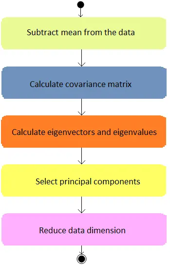
The following diagram summarizes the activities that need to be performed in principal components analysis.
This technique is beneficial for processing data sets with hundreds of variables while maintaining, at the same time, most of the information from the original data set.
Principal components analysis can also be implemented within a neural network. However, as this process is irreversible, the data’s reduction should be done only for the inputs and not for the target variables.