1. Application type.
2. Data set.
3. Neural network.
4. Training strategy.
5. Model selection.
6. Testing analysis.
7. Model deployment.
8. Tutorial video.

1. Application type

2. Data set

The data set contains three concepts:

• Data source.
• Variables.
• Instances.

Data source

The ObesityDataSet.csv file contains the data for this application.

The number of instances (rows) in the data set is 2111, and the number of variables (columns) is 17.

Variables

The number of input variables, or attributes for each sample, is 14. Height and weight are unused variables related to the target variable. The input variables are numeric-valued, binary, and categorical. The number of target variables is 1 and represents the estimation of obesity levels in individuals.

The following list summarizes the variables information:

• gender: (1=Female or 0=Male).
• age: (Numeric).
• height: (Numeric).
• weight: (Numeric).
• family_history_with_overwight: (1=Yes/0=No).
• caloric_food:(0=Yes/1=No). Frequent consumption of high-caloric food.
• vegatables: (1, 2 or 3). Frequency of consumption of vegetables.
• number_meals: (1, 2, 3 or 4). The number of main meals.
• food_between_meals: (1=No, 2=Sometimes, 3=Frequently or 4=Always). Consumption of food between meals.
• smoke: (0=Yes/1=No).
• water: (1, 2 or 3). Consumption of water daily.
• calories: (0=Yes/1=No).Calories consumption monitoring.
• activity: (0, 1, 2 or 3). Physical activity frequency.
• technology: (0, 1 or 2). Time using technology devices.
• alcohol: (1=No, 2=Sometimes, 3=Frequently or 4=Always). Consumption of alcohol.
• transportation: (Automobile, motorbike, bike, public transportation or walking). Transportation used.
• obesity_level: (1=Insufficient_Weight, 2=Normal_Weight, 3=Overweight_Level_I, 4=Overweight_Level_II, 5=Obesity_Type_I, 6=Obesity_Type_II, 7=Obesity_Type_III)

Instances

Finally, the use of all instances is set.

Note that each instance contains a different patient’s input and target variables. The data set is divided into training, validation, and testing subsets. 60% of the instances will be assigned for training, 20% for generalization, and 20% for testing. More specifically, 1267 samples are used here for training, 422 for selection, and 422 for testing samples.

Variables distributions

Once the data set has been set, we are ready to perform a few related analytics. We check the provided information and ensure the data is of good quality. We can calculate the distributions of the variables.

The following chart shows the histogram for the obesity level.

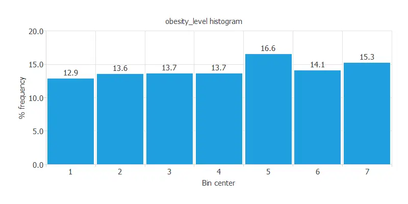
As we can see, the obesity level has a semi-normal distribution. The maximum frequency is 16.6272%, corresponding to the bin with center 5. The minimum frequency is 12.8849%, corresponding to the bin with center 1.

Inputs-targets correlations

The inputs-targets correlations might indicate what factors most influence patients’ obesity level.

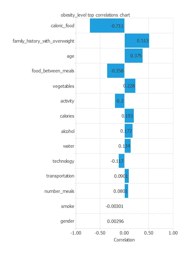
The most correlated variables with obesity are caloric food, family_history_with_overweight, and age.

3. Neural network

The third step is to set the model parameters. Approximation models usually contain the following layers:

• Scaling layer.
• Perceptron layers.
• Unscaling layer.

We set the mean and standard deviation as the scaling method and the minimum and maximum as the unscaling method. The activation function we choose for this model is the hyperbolic tangent activation function and the linear activation function for the hidden and output layers, respectively.

The next figure is a graphical representation of this neural network.

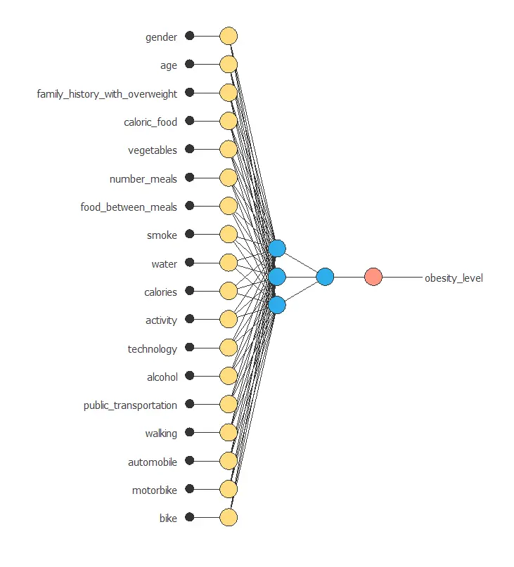
It contains a scaling layer, two perceptron layers, and an unscaling layer.

The number of inputs is 18, and the number of outputs is 1. The complexity, represented by the number of neurons in the hidden layer, is 3.

4. Training strategy

The fourth step is to set the training strategy, which is composed of two terms:

• A loss index.
• An optimization algorithm.

The learning problem can be stated as finding a neural network that minimizes the loss index. That is a neural network that fits the data set (error term) and does not oscillate (regularization term). The loss index is the normalized squared error with L1 regularization. The optimization algorithm that we use is the quasi-Newton method. This is also the standard optimization algorithm for this type of problem.

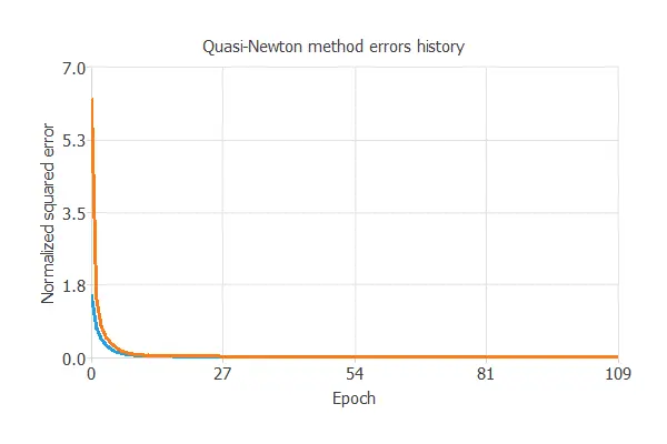
This chart shows how errors decrease with the iterations during training.

The final training and selection errors are training error = 0.0176 WSE and selection error = 0.0236 WSE, respectively.

5. Model selection

The objective of model selection is to improve the generalization capabilities of the neural network or, in other words, to reduce the selection error.

Since the selection error we have achieved is very small (0.0236 NSE), we don’t need to apply order selection or input selection here.

6. Testing analysis

Once the model is trained, we perform a testing analysis to validate its prediction capacity. This will be done by comparing the neural network outputs against the real target values for a data set never seen before.

The testing analysis will determine if the model is ready to move to the production phase.

Linear regression analysis

The next chart illustrates the linear regression analysis for the variable particles_adhering.

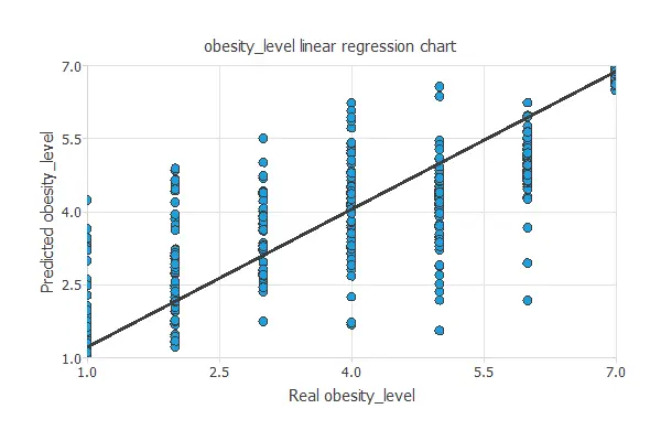
The intercept, slope, and correlation values should be 0, 1, and 1 for a perfect fit. In this case, we have intercept = 0.263, slope = 0.947, and correlation = 0.844.

The achieved values are close to ideal, so the model performs well.

7. Model deployment

Once the neural network’s generalization performance has been tested, the neural network can be saved for future use in the so-called model deployment mode.

Neural network outputs

We can treat new patients by calculating the neural network outputs.

For that, we need to know the patients’ next details. Here we have a new patient:

• gender: Male.
• age: 35.
• family_history_with_overwight: Yes.
• caloric_food: Yes.
• vegatables: 2.
• number_meals: 2.
• food_between_meals: No.
• smoke: Yes.
• water: 2.
• calories: Yes.
• activity: 1.
• technology: 1.
• alcohol: Frequently.
• transportation: public_transportation.
• obesity_level: 5.406 = Obesity_Type_I.

Directional outputs

We can plot directional outputs to study the behavior of the output variable obesity_level as the function of single inputs.

As we see in calculating correlations, weight and height are the inputs that most influence obesity_level. If patients’ height increases, obesity level decreases, and the inverse happen with the weight.

Despite those two attributes, this patient can reduce their obesity level by changing two of her habits. As the obesity level is not a problem that can be solved from one day to another, the treatment must be applied little by little.

The treatment will increase the number of food between meals and have more activity. We can see it below:

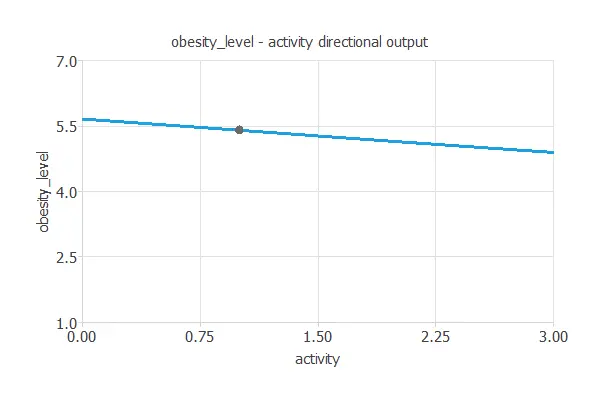
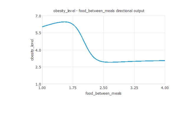
The first plot shows the output obesity level as a function of the input activity. The second one represents the output obesity level as a function of the input food between meals.

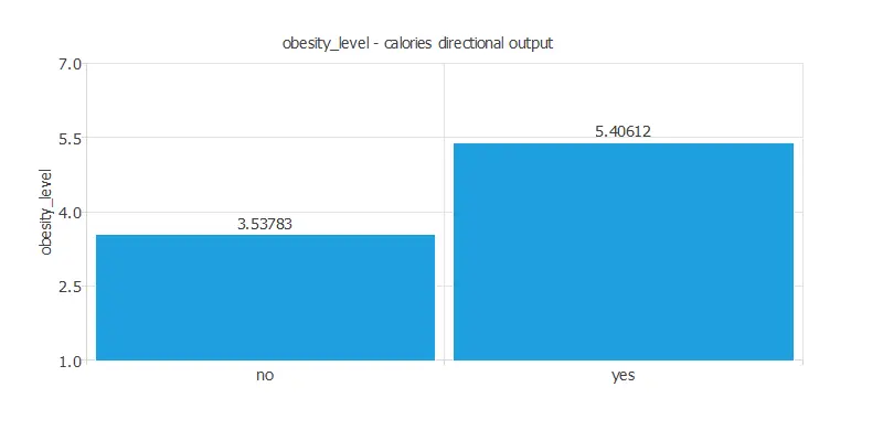
The last graph represents that if the patient consumes more calories, the obesity level is higher.

To sum up, the treatment for this patient is:

• increase the number of food between meals
• more activity such as walking at least 30mins each day
• decrease calories consumption monitoring

Mathematical expression

Besides, we can use the mathematical expression of the neural network, which is listed next.

scaled_gender = (gender-(0.4940789938))/0.5000830293;
scaled_age = age*(1+1)/(61-(14))-14*(1+1)/(61-14)-1;
scaled_family_history_with_overweight = family_history_with_overweight*(1+1)/(1-(0))-0*(1+1)/(1-0)-1;
scaled_caloric_food = (caloric_food-(0.1160589978))/0.320371002;
scaled_vegetables = (vegetables-(2.419039965))/0.5339270234;
scaled_number_meals = number_meals*(1+1)/(4-(1))-1*(1+1)/(4-1)-1;
scaled_food_between_meals = (food_between_meals-(2.140690088))/0.4685429931;
scaled_smoke = smoke*(1+1)/(1-(0))-0*(1+1)/(1-0)-1;
scaled_water = (water-(2.008009911))/0.6129530072;
scaled_calories = calories*(1+1)/(1-(0))-0*(1+1)/(1-0)-1;
scaled_activity = (activity-(1.01030004))/0.8505920172;
scaled_technology = (technology-(0.6578660011))/0.6089270115;
scaled_alcohol = (alcohol-(1.731410027))/0.5154979825;
scaled_public_transportation = (public_transportation-(0.7484599948))/0.4340009987;
scaled_walking = walking*(1+1)/(1-(0))-0*(1+1)/(1-0)-1;
scaled_automobile = (automobile-(0.2164849937))/0.4119459987;
scaled_motorbike = motorbike*(1+1)/(1-(0))-0*(1+1)/(1-0)-1;
scaled_bike = bike*(1+1)/(1-(0))-0*(1+1)/(1-0)-1;
perceptron_layer_0_output_0 = tanh[ -1.16742 + (scaled_gender*0.68282)+ (scaled_age*-0.420455)+ (scaled_family_history_with_overweight*0.691903)+ (scaled_caloric_food*-0.244554)+ (scaled_vegetables*0.769029)+ (scaled_number_meals*0.546811)+ (scaled_food_between_meals*-0.593264)+ (scaled_smoke*-0.250848)+ (scaled_water*-0.00675811)+ (scaled_calories*0.564604)+ (scaled_activity*0.0689401)+ (scaled_technology*0.0396549)+ (scaled_alcohol*-0.0964615)+ (scaled_public_transportation*0.839636)+ (scaled_walking*0.748955)+ (scaled_automobile*0.268782)+ (scaled_motorbike*0.528234)+ (scaled_bike*1.18717) ];
perceptron_layer_0_output_1 = tanh[ 0.32342 + (scaled_gender*-0.195494)+ (scaled_age*0.686579)+ (scaled_family_history_with_overweight*0.0506046)+ (scaled_caloric_food*0.00697568)+ (scaled_vegetables*-0.0795011)+ (scaled_number_meals*-0.0896854)+ (scaled_food_between_meals*0.294397)+ (scaled_smoke*-0.0825197)+ (scaled_water*-0.0133305)+ (scaled_calories*0.0261315)+ (scaled_activity*-0.0911458)+ (scaled_technology*0.010449)+ (scaled_alcohol*0.0786926)+ (scaled_public_transportation*-0.1329)+ (scaled_walking*-0.293047)+ (scaled_automobile*-0.286349)+ (scaled_motorbike*-0.128273)+ (scaled_bike*-0.160357) ];
perceptron_layer_0_output_2 = tanh[ -0.392613 + (scaled_gender*-0.367176)+ (scaled_age*-0.808962)+ (scaled_family_history_with_overweight*-0.384984)+ (scaled_caloric_food*0.131679)+ (scaled_vegetables*-0.0930502)+ (scaled_number_meals*0.221046)+ (scaled_food_between_meals*1.75847)+ (scaled_smoke*0.0215909)+ (scaled_water*-0.178107)+ (scaled_calories*0.513794)+ (scaled_activity*-0.360404)+ (scaled_technology*0.210205)+ (scaled_alcohol*0.451744)+ (scaled_public_transportation*0.289853)+ (scaled_walking*-0.0703812)+ (scaled_automobile*-0.570434)+ (scaled_motorbike*0.979235)+ (scaled_bike*0.448767) ];
perceptron_layer_1_output_0 = [ 0.179259 + (perceptron_layer_0_output_0*1.37047)+ (perceptron_layer_0_output_1*1.60426)+ (perceptron_layer_0_output_2*-0.714662) ];
unscaling_layer_output_0 = perceptron_layer_1_output_0*(7-1)/(1+1)+1+1*(7-1)/(1+1);

The file obesity.py implements the mathematical expression of the neural network in Python.

You can embed this software in any tool to predict new data.

8. Tutorial video

You can watch the step-by-step tutorial video below to help you complete this Machine Learning example

for free using the easy-to-use machine learning software Neural Designer.

References

• We have obtained the data for this problem from the UCI Machine Learning Repository.
• Palechor, F. M., & de la Hoz Manotas, A. (2019). Dataset for estimation of obesity levels based on eating habits and physical condition in individuals from Colombia, Peru and Mexico. Data in Brief, 104344.
• De-La-Hoz-Correa, E., Mendoza Palechor, F., De-La-Hoz-Manotas, A., Morales Ortega, R., & Sanchez Hernandez, A. B. (2019). Obesity level estimation software based on decision trees.

Related posts