
Insurance risk prediction with machine learning is essentially a modeling task: estimate mortality from demographic, medical, and behavioral data. Traditional actuarial methods rely on tables and rule-based scores, but they fail to capture nonlinear relationships and interactions in complex datasets.
With thousands of applicants and hundreds of variables, often incomplete or skewed, the problem is well-suited to machine learning. Neural networks, in particular, can model nonlinearities, handle high-dimensional data, and improve both accuracy and efficiency.
This article presents a case study applying ML to life insurance risk assessment, covering data preparation, model design, and performance evaluation, along with the business impact of moving from manual scoring to advanced analytics.
Contents
Data set
The dataset used here is taken from Kaggle, one of the most important repositories of data science.
It contains information about 60.000 customers with 145 attributes.
This data set contains about 400.000 missing values, i.e., information about customers unavailable to the company.
However, machine learning can deal with incomplete data without problems.
The input variables include personal, family history, medical history, and external variables.
The target variable is the risk of that client. The risk is a subjective variable because it is granted by people, specifically risk analysts.
The following table shows the distribution of the risk evaluations.
| None | 8 |
|---|---|
| Very low | 7 |
| Low | 6 |
| Medium-low | 5 |
| Medium | 4 |
| Medium-high | 3 |
| High | 2 |
| Very high | 1 |
It might be interesting to study how the different features affect a customer’s risk. We can calculate the correlation coefficients between all the inputs and the target.
Correlations close to 1 indicate a high dependency of the target on the input. Correlations close to 0 mean that there is a low dependency. Note that, in general, the targets depend on many inputs simultaneously.
The following images show the absolute value of the linear correlations between all inputs and the target variable.
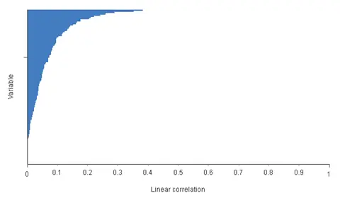
As we can see, the three most influential variables for the risk are the body mass index BMI (0.382), the weight Wt (0.351), and the medical history 23 (0.287).
The next step is to know the distribution of the target variable over its entire range. Box plots display information about the first, second, third, and fourth quartiles of a single variable in the data set. The following chart shows the box plot for the risk.
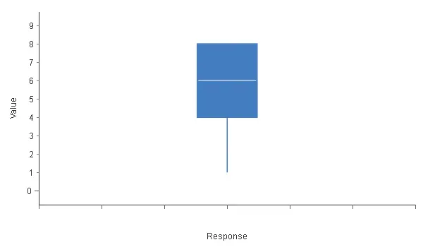
In this case, the Box plot tells us that the minimum risk is 1, the first quartile is 4, the second quartile or median is 6, the third quartile is 8, and the maximum is 8. Note that the upper quartile is missing, which means that the risk variable is not well distributed.
Histograms also give us valuable information on the distribution of a variable. The following chart shows the histogram for the risk.
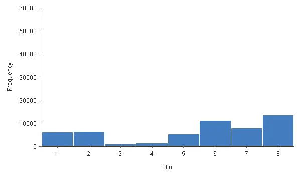
The chart above shows that the most common risk value is 8 (low). The less common risk value is 3 (medium-high). We can see that this histogram does not have a normal (or Gaussian) distribution. Indeed, analysts tend to give either low or high-risk values. The 3 and 4 values have very low frequencies. The value 7 has a lower frequency than the values 6 and 8.
Therefore, the distribution of the target variable is wrong. It should be a normal distribution, but clearly, it is not. Indeed, most customers should have a medium risk. This is because some risk analysts tend to give low or high evaluations.
Our model should output risk values with a normal distribution.
Risk model
The next step of our study is to build a model capable of evaluating our potential customers’ risks. This model will utilize the extensive information provided to us.
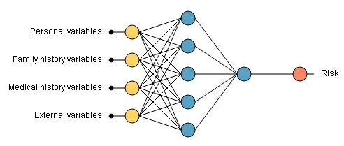
For this purpose, we apply insurance risk prediction with machine learning techniques, specifically neural networks. Neural networks rank among the most powerful methods to discover intricate relationships, recognize complex patterns, and predict trends hidden in the data.For this purpose, we use a technique called neural networks. Neural networks are among the most potent methods to discover intricate relationships, recognize complex patterns, or predict current trends in your data.
The following graph illustrates the neural network used in this application. Note that the neural network is too large to be plotted.
After training the network, we evaluate its performance to check if our risk model helps assess clients. The table below shows the minimums, maximums, means, and standard deviations of the neural network’s absolute, relative, and percentage errors for the testing data.
| Mean absolute error | 1.534 |
|---|---|
| Mean percentage error | 21.920% |
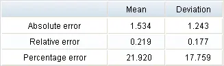
As we can see, the mean error is 1.5 over 8. That means the model evaluates customers’ risk with quite a high precision.
Now, let’s look at the histogram of the risk variable by applying the predictive model.
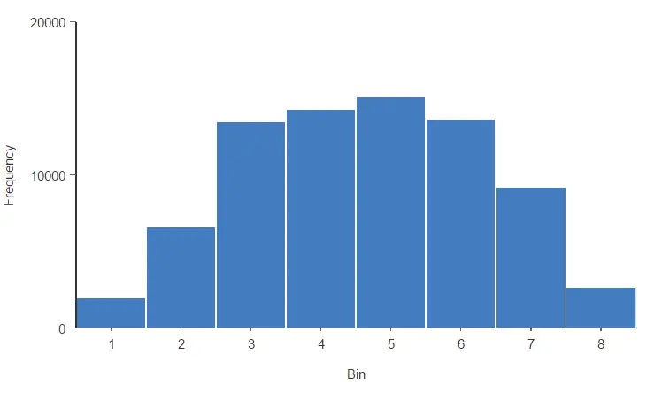
The previous histogram indicates that the risk variable now follows a normal distribution, indicating it is well distributed.
Most customers have average values, and the evaluations do not focus on the extremes. This is a desirable property of our risk model.
Conclusions
This case study shows how insurance risk prediction with machine learning reshapes the way insurers evaluate applicants: we prepare high-dimensional data, extract key features, and train neural networks that outperform traditional actuarial scoring. The benefits go beyond accuracy, these models deliver faster, more consistent evaluations while cutting operational costs from manual underwriting, lengthy review cycles, and avoidable errors.