An insurance company has provided health insurance to its customers. Now, they want to predict whether the customers from past years will also be interested in vehicle insurance provided by the company.

Customer targeting consists of identifying those persons that are more prone to a specific product or service.

Contents

1. Application type.
2. Data set.
3. Neural network.
4. Training strategy.
5. Model selection.
6. Testing analysis.
7. Model deployment.
8. Tutorial video.

This example is solved with Neural Designer. In order to follow this example step by step, you can use the free trial.

1. Application type

This is a classification project since the predictor variable is binary (interested or not interested).

The goal here is to create a model to obtain the probability of being interested as a function of customer features.

2. Data set

The data set contains information to create our model. We need to configure three things:

• Data source.
• Variables.
• Instances.

The data file used for this example is vehicle-insurances.csv, which contains 9 features about 381109 customers of the insurance company.

The data set includes the following variables:

• id: unique ID for the customer.
• gender: gender of the customer.
• age: age of the customer.
• previously_insured: yes = customer already has vehicle insurance, no = customer doesn’t have vehicle insurance
• vehicle_age: age of the Vehicle.
• vehicle_damage: yes = customer got his/her vehicle damaged in the past, no = customer didn’t get his/her vehicle damaged in the past.
• annual_premium: the amount the customer needs to pay as a premium in the year.
• vintage: number of days the customer has been associated with the company.
• response: interested = customer is interested, not-interested = customer is not interested.

On the other hand, the instances are divided randomly into training, selection, and testing subsets, containing 60%, 20%, and 20% of the instances, respectively.

Our target variable is the response. We can calculate the data distributions and plot a pie chart with the percentage of instances for each class.

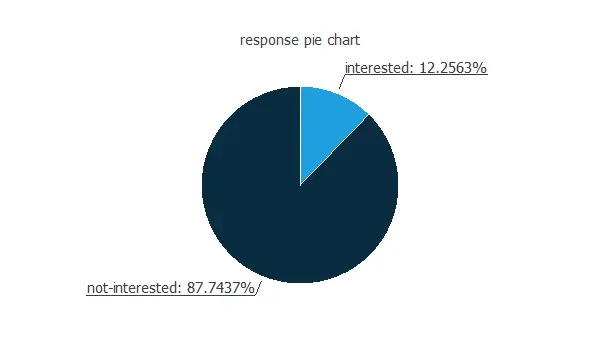
As we can see, the target variable is very unbalanced since many customers are not interested in vehicle insurance, almost 88%, while only 12% are interested. Therefore, we could say that around 1 out of 10 customers are interested in vehicle insurance.

Furthermore, we can also compute the inputs-target correlations, which might indicate which factors have the most significant influence on vehicle insurance.

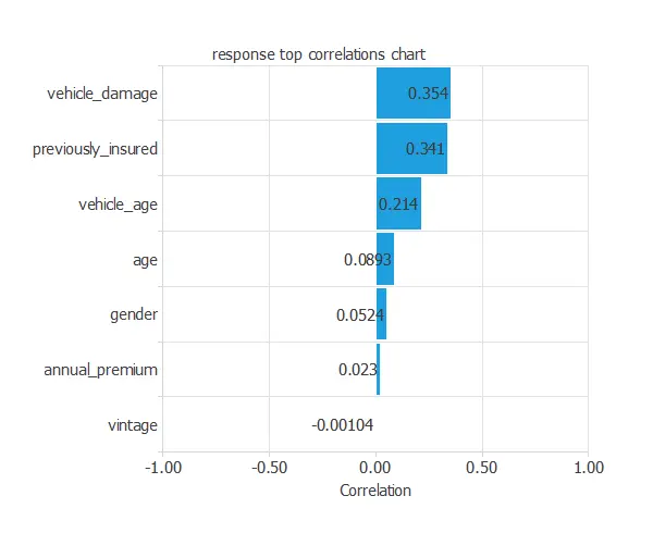
In this example, vehicle_damage and previously_insured are the two variables with the highest correlation, vehicle_damage has a positive correlation, while previously_insured has a negative correlation.

3. Neural network

The next step is to set the neural network parameters. For classification problems, it is composed of:

• Scaling layer.
• Perceptron layers.
• Probabilistic layer.

For the scaling layer, the mean and standard deviation scaling method has been set.

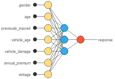
We set one perceptron layer with 3 neurons having the logistic activation function. This layer has seven inputs, and since the target variable is binary, only one output.

The neural network for this example can be represented with the following diagram:

4. Training strategy

The fourth step is to set the training strategy, which defines what the neural network will learn. A general training strategy for classification is composed of two terms:

• A loss index.
• An optimization algorithm.

The loss index chosen for this problem is the normalized squared error between the outputs from the neural network and the targets in the data set with L1 regularization.

The selected optimization algorithm is the adaptative linear momentum.

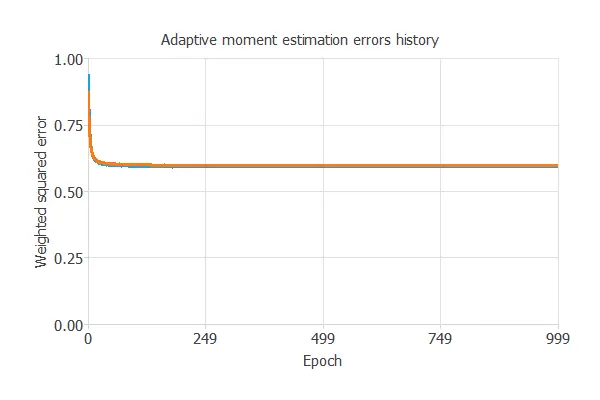
The following chart shows how the training and selection errors develop with the epochs during the training process. The final values are training error = 0.593 NSE and selection error = 0.598 NSE.

5. Model selection

The objective of model selection is to find the network architecture with the best generalization properties, which means finding the one that minimizes the error on the selected instances of the data set.

More specifically, we want to find a neural network with a selection error of less than 0.598 NSE, which is the value that we have achieved so far.

Order selection algorithms train several network architectures with a different number of neurons and select the one with the smallest selection error.

The incremental order method starts with a few neurons and increases the complexity at each iteration.

The final selection error achieved is 0.5873 for an optimal number of neurons of 6.

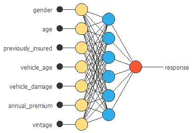
The graph above represents the architecture of the final neural network.

6. Testing analysis

The objective of the testing analysis is to validate the generalization performance of the trained neural network.

To validate a classification technique, we need to compare the values provided by this technique to the observed values. We can use the ROC curve as it is the standard testing method for binary classification projects.

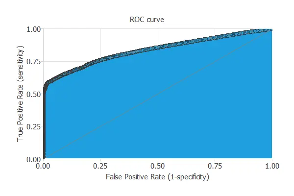
The AUC value for this example is 0.8342.

The following table contains the elements of the confusion matrix. This matrix contains the true positives, false positives, false negatives and true negatives for the variable response.

The total number of testing samples is 76221. The number of correctly classified samples is 48519 (63%), and the number of misclassified samples is 27702 (36%).

We are interested in the customers classified as positive (first column); if we only contacted 47% of the total number of customers (those predicted as positive), the ratio of interested customers would be approximately 1 out of every five contacts, which doubles the ratio obtained if we contacted the whole sample (1 out of 10). Moreover, the number of true positives classified as negative (customers interested but we would not contact) is deficient, 205 out of 76221 (0.27%).

We can also observe these results in the positive rates chart:

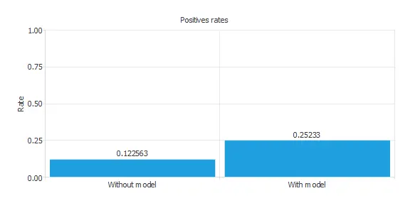
The initial positive rate was around 12%, and now, after applying our model, it is 25%. This means that we would be able to duplicate the vehicle insurance sales with this model.

We can also perform the cumulative gain analysis, which is a visual aid that shows the advantage of using a predictive model as opposed to randomness.

It consists of three lines. The baseline represents the results that would be obtained without using a model. The positive cumulative gain shows in the y-axis the percentage of positive instances found against the population represented in the x-axis.

Similarly, the negative cumulative gain shows the percentage of the negative instances found against the population percentage.

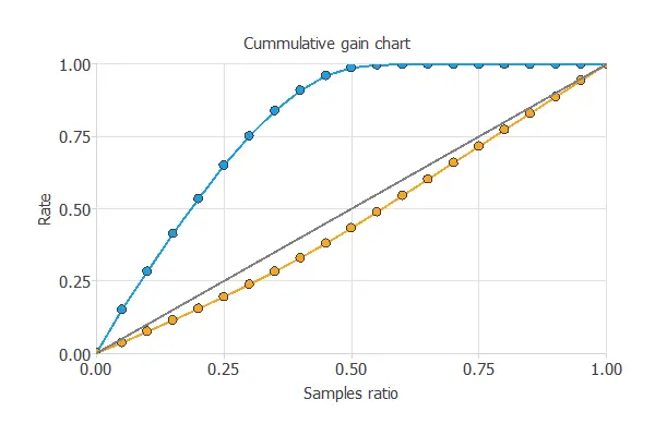
In this case, by using the model, we see that by analyzing 50% of the clients with a higher probability of being interested in the vehicle insurance, we would reach almost 100% of clients that would take out the insurance.

Another testing method is the profit chart.
This testing method shows the difference in profits from randomness and those using the model depending on the instance ratio.

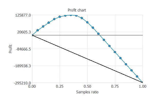
The values of the previous plot are displayed below:

• Unitary cost: 10 USD
• Unitary income: 50 USD
• Maximum profit: 125877 USD
• Samples ratio: 0.35

In the graph, we can observe that having a unitary cost of 10 USD and a unitary income of 50 USD, if we contact 35% of the customers most likely to be interested in the vehicle insurance, we would have the maximum benefit (125877 USD).

7. Model deployment

The model obtained after all the steps is not the best it could be achieved. Nevertheless, it is still better than guessing randomly.

The objective of the Response Optimization algorithm is to exploit the mathematical model to look for optimal operating conditions. Indeed, the predictive model allows us to simulate different operating scenarios and adjust the control variables to improve efficiency.

An example is to maximize response probability while maintaining the age between two desired values.

The next table resumes the conditions for this problem.

The next list shows the optimum values for previous conditions.

• gender: female.
• age: 44.
• previously_insured: 1 (yes).
• vehicle_age: 3.
• vehicle_damage: 1 (yes).
• annual_premium: 85848.8.
• vintage: 204.
• response: 80%.

The next listing shows the mathematical expression of the predictive model.

scaled_gender = gender*(1+1)/(1-(0))-0*(1+1)/(1-0)-1;
scaled_age = age*(1+1)/(85-(20))-20*(1+1)/(85-20)-1;
scaled_previously_insured = previously_insured*(1+1)/(1-(0))-0*(1+1)/(1-0)-1;
scaled_vehicle_age = vehicle_age*(1+1)/(3-(1))-1*(1+1)/(3-1)-1;
scaled_vehicle_damage = vehicle_damage*(1+1)/(1-(0))-0*(1+1)/(1-0)-1;
scaled_annual_premium = annual_premium*(1+1)/(540165-(2630))-2630*(1+1)/(540165-2630)-1;
scaled_vintage = vintage*(1+1)/(299-(10))-10*(1+1)/(299-10)-1;

perceptron_layer_output_0 = tanh[ -0.233398 + (scaled_gender*-0.442383)+ (scaled_age*0.807861)+ (scaled_previously_insured*0.963257)+ (scaled_vehicle_age*-0.937439)+ (scaled_vehicle_damage*-0.78479)+ (scaled_annual_premium*-0.0365601)+ (scaled_vintage*-0.572449) ];
perceptron_layer_output_1 = tanh[ -0.724854 + (scaled_gender*0.927185)+ (scaled_age*0.696899)+ (scaled_previously_insured*-0.251282)+ (scaled_vehicle_age*-0.990173)+ (scaled_vehicle_damage*0.47937)+ (scaled_annual_premium*-0.197021)+ (scaled_vintage*-0.838135) ];
perceptron_layer_output_2 = tanh[ 0.452454 + (scaled_gender*0.517029)+ (scaled_age*0.893494)+ (scaled_previously_insured*-0.773743)+ (scaled_vehicle_age*0.477539)+ (scaled_vehicle_damage*-0.932251)+ (scaled_annual_premium*-0.0134888)+ (scaled_vintage*0.99707) ];
perceptron_layer_output_3 = tanh[ -0.59967 + (scaled_gender*0.159912)+ (scaled_age*0.602417)+ (scaled_previously_insured*0.937988)+ (scaled_vehicle_age*-0.426086)+ (scaled_vehicle_damage*-0.157532)+ (scaled_annual_premium*0.194153)+ (scaled_vintage*-0.392334) ];
perceptron_layer_output_4 = tanh[ -0.649536 + (scaled_gender*-0.85968)+ (scaled_age*0.686707)+ (scaled_previously_insured*0.222839)+ (scaled_vehicle_age*0.263245)+ (scaled_vehicle_damage*-0.328613)+ (scaled_annual_premium*-0.567871)+ (scaled_vintage*-0.525146) ];
perceptron_layer_output_5 = tanh[ -0.581116 + (scaled_gender*0.530884)+ (scaled_age*-0.667358)+ (scaled_previously_insured*-0.549866)+ (scaled_vehicle_age*-0.768677)+ (scaled_vehicle_damage*-0.619324)+ (scaled_annual_premium*-0.226624)+ (scaled_vintage*-0.885376) ];

probabilistic_layer_combinations_0 = -0.593079 +0.960022*perceptron_layer_output_0 -0.123474*perceptron_layer_output_1 +0.800903*perceptron_layer_output_2 +0.802307*perceptron_layer_output_3 +0.0870361*perceptron_layer_output_4 +0.528748*perceptron_layer_output_5 
    
response = 1.0/(1.0 + exp(-probabilistic_layer_combinations_0);

The company can also embed this formula in any software tool.

8. Video tutorial

You can watch the step by step tutorial video below to help you complete this Machine Learning example
for free using the powerful machine learning software, Neural Designer.

References

• The data for this problem has been taken from the Machine Learning Repository Kaggle.

Related posts