
Model next-month payment default
Use the UCI Default of Credit Card Clients dataset to classify the next monthly payment outcome. The saved network uses 23 inputs and is evaluated on 6,000 held-out customer records.
1. Business decision
Credit analysts can study how historical repayment and account descriptors associate with next-month default. The example demonstrates benchmark evaluation and error trade-offs; it does not estimate fraud or prescribe a lending decision.
Payment outcome
Keep next-month default distinct from transaction fraud.
Error trade-off
Review default sensitivity and false-positive costs.
Portfolio validation
Compare performance on later customer cohorts.
2. Data set
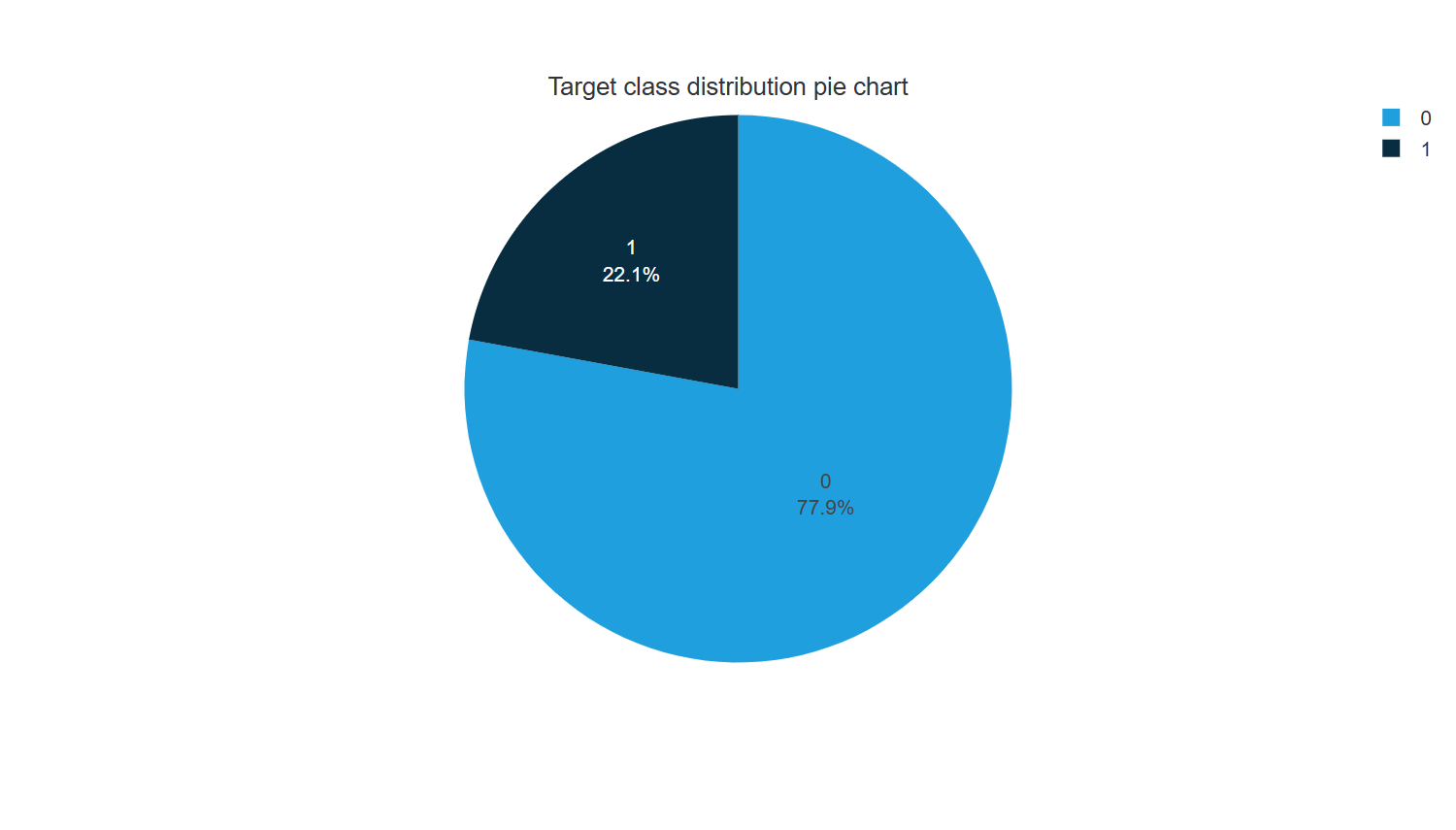
The dataset contains 30,000 credit-card customer records. The identifier is excluded, and the target default_payment_next_month uses 1 for default and 0 for no default.
Source: Default of Credit Card Clients. Dataset license: CC-BY-4.0. The downloadable ZIP includes the adapted data and attribution notices.
| Dataset measure | Saved value |
|---|---|
| Analysis unit | customer record |
| Records | 30,000 |
| Raw variables | 24 |
| Encoded model inputs | 23 |
| Model outputs | 1 |
| Training roles | 18000 |
| Validation / selection roles | 6000 |
| Testing roles | 6000 |
| Unused roles | 0 |
| Field | Role | Type | Categories |
|---|---|---|---|
| LIMIT_BAL | Input | Numeric | |
| SEX | Input | Numeric | |
| EDUCATION | Input | Numeric | |
| MARRIAGE | Input | Numeric | |
| AGE | Input | Numeric | |
| PAY_0 | Input | Numeric | |
| PAY_2 | Input | Numeric | |
| PAY_3 | Input | Numeric | |
| PAY_4 | Input | Numeric | |
| PAY_5 | Input | Numeric | |
| PAY_6 | Input | Numeric | |
| BILL_AMT1 | Input | Numeric | |
| BILL_AMT2 | Input | Numeric | |
| BILL_AMT3 | Input | Numeric | |
| BILL_AMT4 | Input | Numeric | |
| BILL_AMT5 | Input | Numeric | |
| BILL_AMT6 | Input | Numeric | |
| PAY_AMT1 | Input | Numeric | |
| PAY_AMT2 | Input | Numeric | |
| PAY_AMT3 | Input | Numeric | |
| PAY_AMT4 | Input | Numeric | |
| PAY_AMT5 | Input | Numeric | |
| PAY_AMT6 | Input | Numeric | |
| default_payment_next_month | Target | Binary | 0, 1 |
3. Model
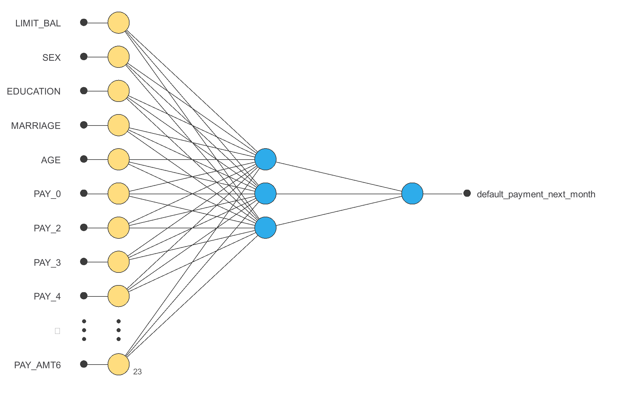
The model has 23 encoded inputs and 1 outputs. No architecture-selection experiment is recorded in this project. The diagram shows the topology used by the saved model.
| Layer | Input shape | Output shape | Activation |
|---|---|---|---|
| Scaling | 23 | 23 | |
| Dense | 23 | 3 | Tanh |
| Dense | 3 | 1 | Sigmoid |
Output values are uncalibrated model scores. For binary evaluation, the saved positive class is 1.
4. Training strategy
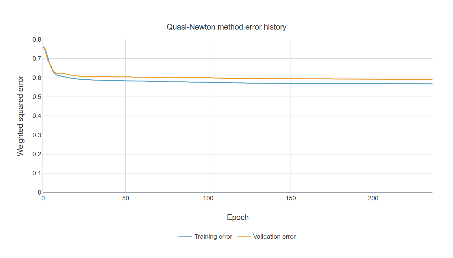
The saved training configuration uses QuasiNewton with WeightedSquaredError.
Quasi-Newton method results
| Measure | Value |
|---|---|
| Epochs number | 237 |
| Elapsed time | 00:00:02 |
| Stopping criterion | Minimum loss decrease |
| Training error | 0.568 |
| Validation error | 0.591 |
5. Model selection
No model selection experiment is recorded for this version. The validation subset guides fitting where a training report is present; it is distinct from the held-out test rows.
On this test subset a majority-class baseline would correctly classify 78.07% of the records. This baseline does not detect both classes and is not an optimized model.
6. Testing analysis
The figures and tables below refer to the current project’s saved testing analysis. The subset uses testing role 2; it contains 6000 source records.
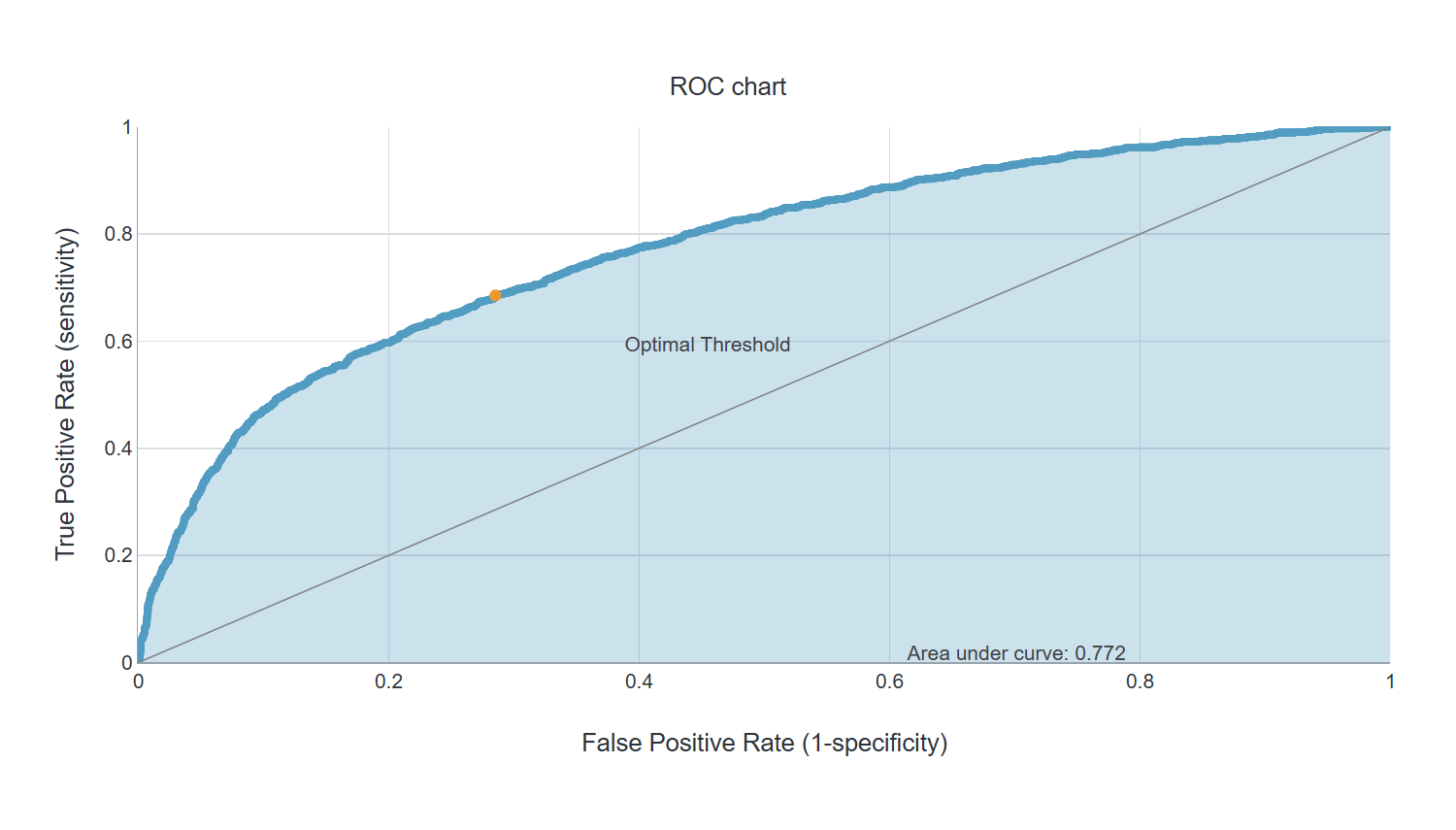
ROC AUC describes ranking on this testing subset. Any optimal threshold shown in the saved ROC report was selected descriptively on that same subset; it is not an independently validated operating policy.
These operating-point metrics are calculated from the saved confusion counts at threshold 0.5. The positive-label coding is stated in the model section.
Confusion table
| Measure | Predicted positive | Predicted negative | Total |
|---|---|---|---|
| Actual positive | 792 (13.2%) | 524 (8.7%) | 1316 (21.9%) |
| Actual negative | 954 (15.9%) | 3730 (62.2%) | 4684 (78.1%) |
| Total | 1746 (29.1%) | 4254 (70.9%) | 6000 (100.0%) |
| Test measure | Value |
|---|---|
| Testing records | 6000 |
| Positive cases | 1316 |
| Positive prevalence | 21.93% |
| Accuracy | 75.37% |
| Sensitivity / recall | 60.18% |
| Specificity | 79.63% |
| Precision / PPV | 45.36% |
| F1 score | 0.517 |
Area under curve
| Measure | Value |
|---|---|
| Area under curve | 0.772 |
7. Model deployment
Open the downloaded project in Neural Designer, inspect the dataset roles and preprocessing, then review the saved task report. Use the same input schema and category order when calculating outputs. The ZIP contains the exact current .nd, its source data and the applicable dataset notices.
Workflow: source measurements → schema and availability checks → model output → domain review. Keep model versions, validation evidence and incoming-data monitoring together.
8. Evidence and limitations
Internal row-level evaluation does not establish current portfolio performance, calibration or fair treatment across groups. Historical selection, policy and economic changes may shift the result. Human review and independent temporal, subgroup and calibration evaluation are required before individual lending decisions.
References
- Default of Credit Card Clients. I-Cheng Yeh. 10.24432/C55S3H
- Dataset terms: Creative Commons Attribution 4.0 International. Full attribution and transformations are included in
LICENSES/DATASET-LICENSE.txt. - Current Neural Designer project and saved task report, snapshot 6 October 2026.