TensorFlow and Neural Designer are popular machine learning platforms developed by Google and Artelnics, respectively.
Although all those frameworks are based on neural networks, they present essential differences in functionality, usability, performance, consumption, etc.
This post compares the energy consumption of TensorFlow and Neural Designer using the GPU for an approximation benchmark.
As we will see, Neural Designer consumes 42% less than its competitor machine learning platform.
In this article, we outline all the steps required to reproduce the results using Neural Designer (download)
Contents:
Introduction
Two of the most essential features of machine learning platforms are their training speed and the total amount of energy consumed during this process.
In most cases, modeling huge data sets is very expensive in computational terms, which leads to a high economic cost of neural network training and a high environmental impact.
Thus, this article aims to measure the GPU energy consumption of TensorFlow and Neural Designer for a benchmark application. Also, a couple of instructions are given to enable anyone to repeat this one or a similar benchmark and check on their own the fantastic results obtained when Neural Designer is used.
The following table summarizes the technical features of these tools that might impact their GPU performance.
| TensorFlow | Neural Designer | |
|---|---|---|
| Written in | C++, CUDA, Python | C++, CUDA |
| Interface | Python | Graphical User Interface |
| Differentiation | Automatic | Analytical |
The above table shows that TensorFlow is programmed in C++ and Python, whereas Neural Designer is entirely programmed in C++.
Interpreted languages like Python have advantages over compiled languages like C ++, such as their ease of use.
However, the performance of Python is generally lower than that of C++. Indeed, Python takes significant time to interpret sentences during the program’s execution.
On the other hand, TensorFlow uses automatic differentiation, while Neural Designer uses analytical differentiation.
As before, automatic differentiation has some advantages over analytical differentiation. Indeed, it simplifies obtaining the gradient for new architectures or loss indices.
However, the performance of automatic differentiation is, in general, lower than that of analytical differentiation:
The first derives the gradient during the program’s execution, while the second has that formula pre-calculated.
Next, we use TensorFlow and Neural Designer to measure the energy consumption for a benchmark problem on a reference computer. The results produced by these platforms are then compared.
Benchmark application
The first step is to choose a benchmark application that is general enough to conclude the performance of the machine learning platforms. As previously stated, we will train a neural network that approximates a set of input-target samples.
In this regard, an approximation application is defined by a data set, a neural network, and an associated training strategy.
The following table uniquely defines these three components.
Data set |
|
|---|---|
Neural network |
|
Training strategy |
|
Once the TensorFlow and Neural Designer applications have been created, we must run them.
Reference computer
The next step is to choose the computer in which the neural network will be trained with TensorFlow and Neural Designer.
The table below shows the features of the computer used for this instance.
| Operating system: | Windows 11 Home 64-bit |
|---|---|
| Processor: | Intel(R) Core(TM) i7-8700 CPU @ 3.20GHz, 3192 Mhz, 6 Core(s), 12 Logical Processor(s) |
| Physical RAM: | 31.9 GB |
| Device (GPU): | NVIDIA GeForce GTX 1050 Ti |
Once the computer has been selected, we install TensorFlow (2.1.0) and Neural Designer (5.9.9) on it.
Below, the TensorFlow code used is shown.
import tensorflow as tf
import pandas as pd
import time
import numpy as np
from tensorflow.keras.utils import Sequence

#read data float32


filename = "C:/Users/Usuario/Downloads/rosenbrock.csv"
df_test = pd.read_csv(filename, nrows=100)
float_cols = [c for c in df_test if df_test[c].dtype == "float64"]
float32_cols = {c: np.float32 for c in float_cols}
data = pd.read_csv(filename, engine='c', dtype=float32_cols)


x = data.iloc[:,:-1].values
y = data.iloc[:,[-1]].values

initializer = tf.keras.initializers.RandomUniform(minval=-1., maxval=1.)


#build model

model = tf.keras.models.Sequential([tf.keras.layers.Dense(1000,activation = 'tanh', kernel_initializer = initializer, bias_initializer=initializer),
tf.keras.layers.Dense(1, activation = 'linear', kernel_initializer = initializer, bias_initializer=initializer)])


#compile model

model.compile(optimizer='adam', loss = 'mean_squared_error')


#train model

class DataGenerator(Sequence):
                def __init__(self, x_set, y_set, batch_size):
                self.x, self.y = x_set, y_set
                self.batch_size = batch_size

                def __len__(self):
                return int(np.ceil(len(self.x) / float(self.batch_size)))

                def __getitem__(self, idx):
        batch_x = self.x[idx * self.batch_size:(idx + 1) * self.batch_size]
        batch_y = self.y[idx * self.batch_size:(idx + 1) * self.batch_size]
                return batch_x, batch_y

train_gen = DataGenerator(x, y, 1000)

start_time = time.time()
with tf.device('/gpu:0'):
    history = model.fit(train_gen, epochs=20000)
print("Training time: ", round(time.time() - start_time), " seconds")
Reference electricity consumption meter
This section describes the device used for the energy consumption measurements so that the reader can reproduce the results obtained in the following section with maximum accuracy.
| Device model | Perel E305EM5-G |
|---|
Results
The last step is to run the benchmark application on the selected machine with TensorFlow and Neural Designer and compare the energy consumed by those platforms during training.
The following figure shows the training time with TensorFlow.
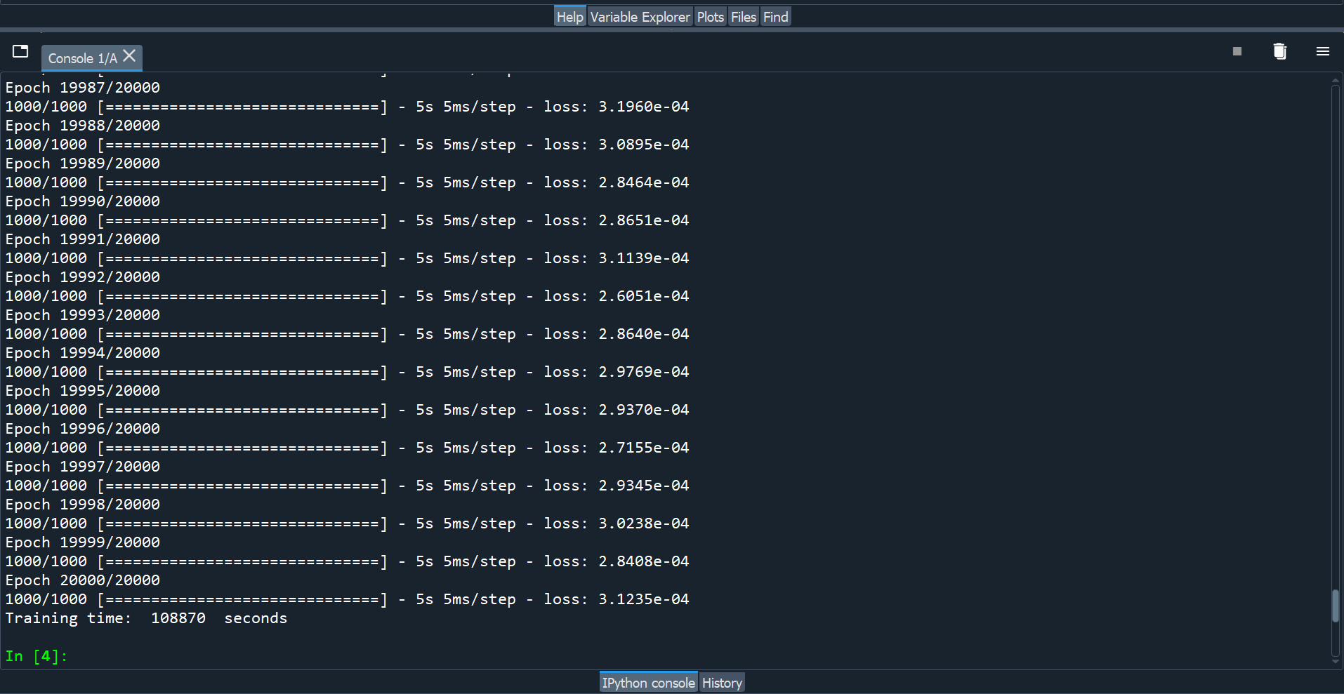
As we can see, TensorFlow takes 30:14:30 to train the neural network for 20000 epochs (5.44 seconds/epoch).
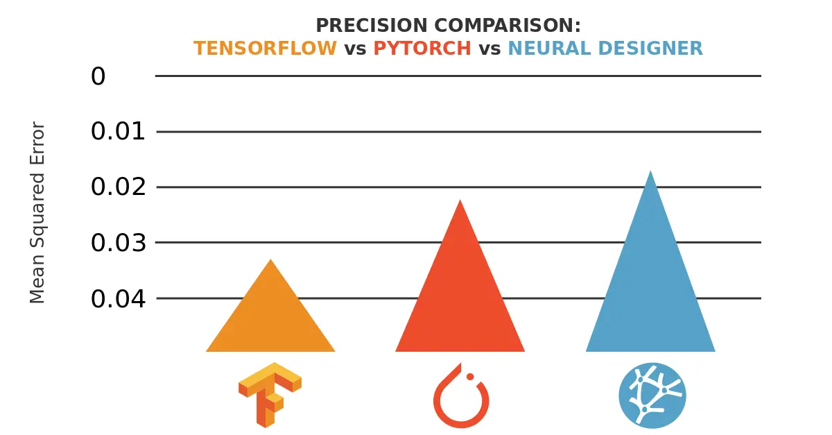
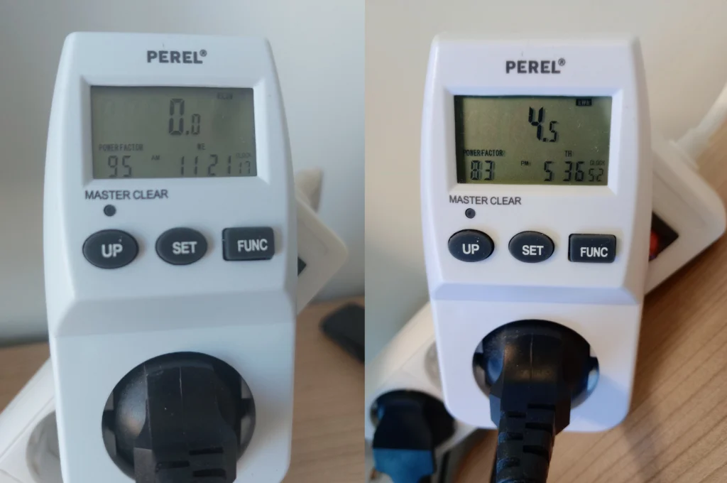
The final mean squared error is 0.0003. The overall energy consumption of the training process is 4.5 kWh, as shown below.
Finally, the following figure shows the training time with Neural Designer.
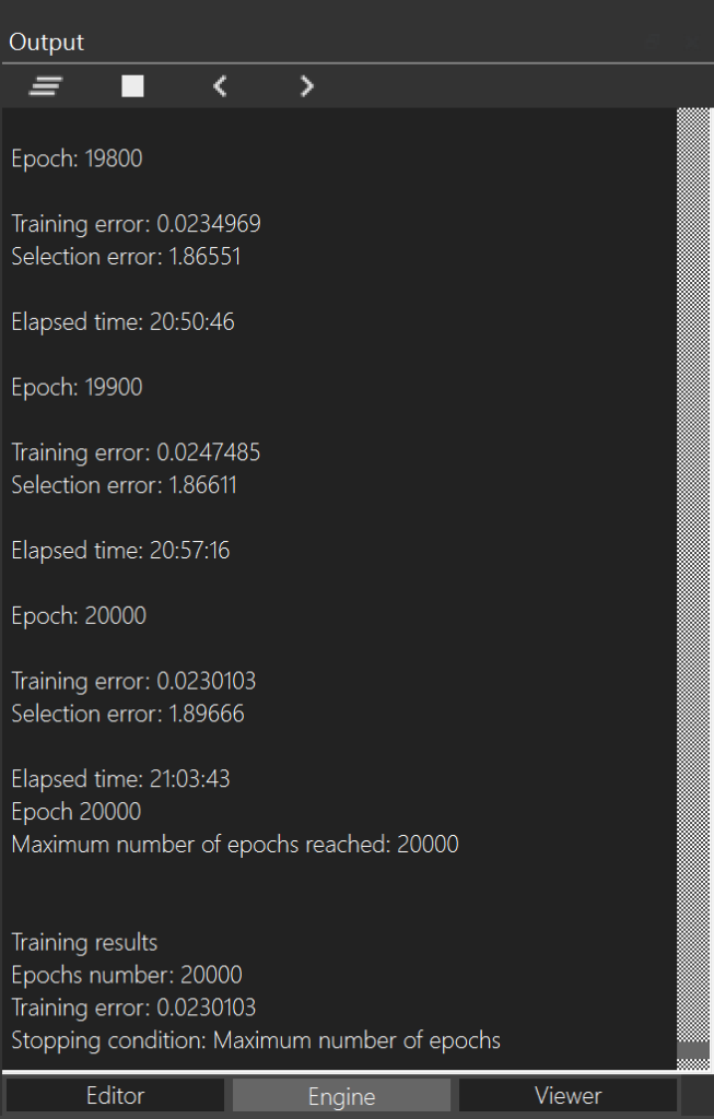
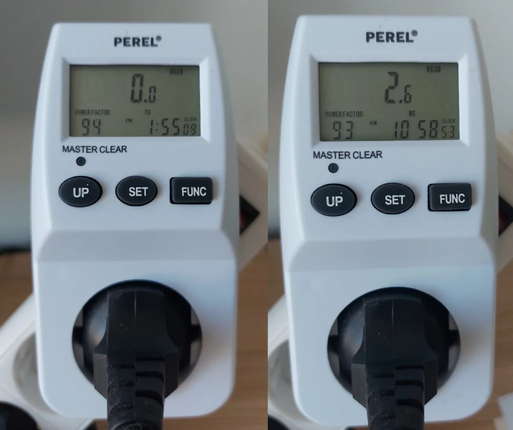
Neural Designer takes 21:03:43 to train the neural network for 20000 epochs (3.79 seconds/epoch). During that time, it reaches a mean squared error of 0.023. The overall energy consumption of the training process is 2.6 kWh, as shown below.
The following table summarizes the the most important metrics the two machine learning platforms yielded.
| TensorFlow | Neural Designer | |
|---|---|---|
| Training time | 30:14:30 | 21:03:43 |
| Epoch time | 5.44 seconds/epoch | 3.79 seconds/epoch |
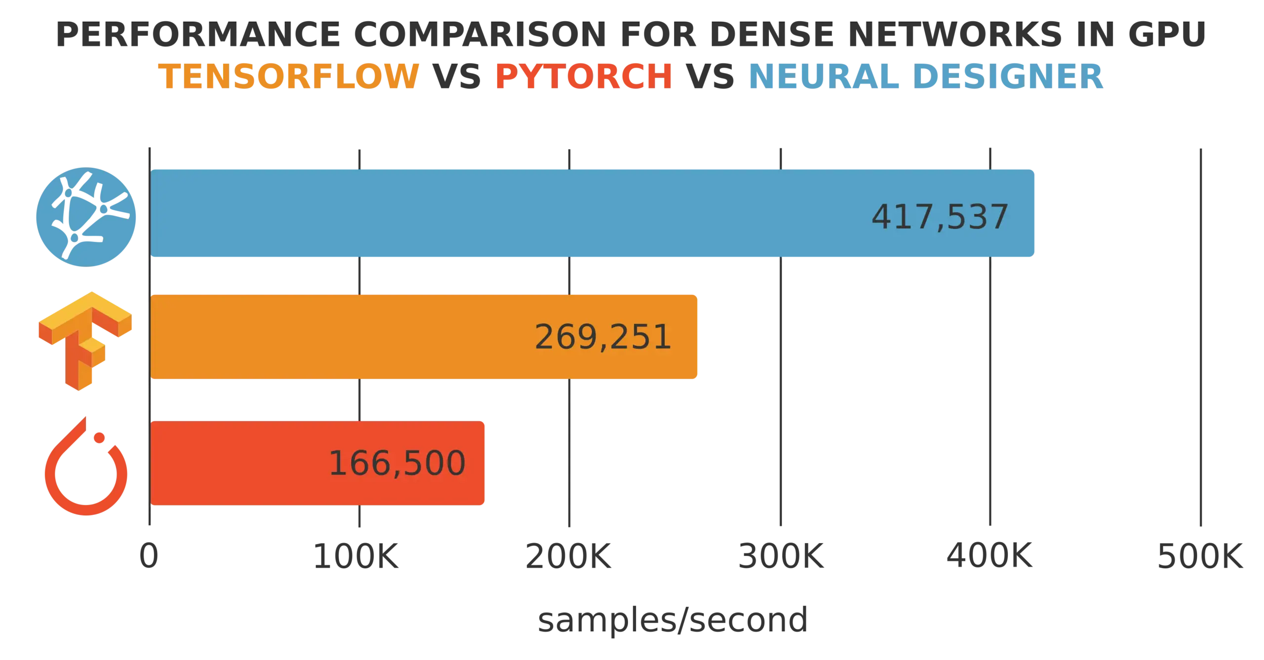
| Training speed | 183,824 samples/second | 263.852 samples/second |
| Total energy consumed | 4.5kWh | 2.6 kWh |
The following chart depicts the energy consumed using TensorFlow and Neural Designer graphically in this case.
Electric energy consumption
Neural Designer
As we can see, the energy consumption of Neural Designer for this application is 42 % lower than that of TensorFlow.
Conclusions
Neural Designer is entirely written in C ++, uses analytical differentiation, and has been optimized to minimize the number of operations during training.
As a result, its energy consumption during the training process using Neural Designer is 42 % lower than that using TensorFlow.
To reproduce these results, download Neural Designer and follow the steps described in this article.