Precision comparison of machine learning platforms: TensorFlow vs PyTorch vs Neural Designer

Platforms

Roberto López
https://es.linkedin.com/in/robertolopezartelnics
August 31, 2023

Training accuracy comparison of machine learning platforms: TensorFlow vs. PyTorch vs. Neural Designer

TensorFlow, PyTorch and Neural Designer
are three popular machine learning platforms developed by
Google,
Facebook and
Artelnics, respectively.

Although all that frameworks implement neural networks,
they present some important differences in functionality, usability, performance, etc.

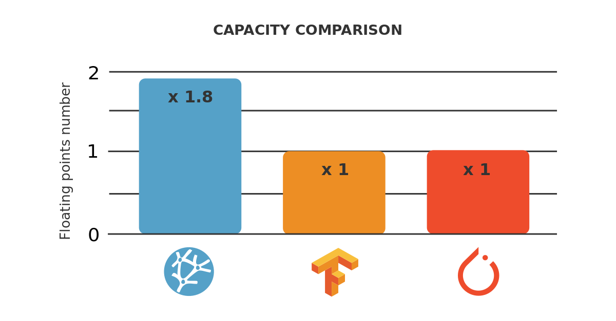
This post compares the training accuracy of TensorFlow, PyTorch, and Neural Designer for an approximation benchmark.

As we will see, the training accuracy of Neural Designer using the Levenberg-Marquardt algorithm is x1.91 higher than that of TensorFlow and x1.21 times higher than that of PyTorch using Adam.

Moreover, Neural Designer trains this neural network x5.71 times faster than TensorFlow and x8.21 times faster than PyTorch.

In this article, we provide all the steps that you need to reproduce the results using the free trial of Neural Designer.

Contents:

Introduction.
Benchmark application.
Reference computer.
Results.
Conclusions.

Introduction

One of the most critical factors in machine learning platforms is their training accuracy.

This article aims to measure the training accuracies of TensorFlow, PyTorch, and Neural Designer for a benchmark application and compare the speeds obtained by those platforms.

The most important factor for training accuracy is the optimization algorithm used.

The above table shows that TensorFlow and PyTorch are programmed in C++ and Python,
while Neural Designer is entirely programmed in C++.

Next, we measure the training accuracy for a benchmark problem on a reference computer using TensorFlow, PyTorch, and Neural Designer.
We then compare the results produced by that platforms.

Benchmark application

The first step is to choose a benchmark application that is general enough to conclude the performance of the machine learning platforms.
As previously stated, we will train a neural network that approximates a set of input-target samples.

In this regard, an approximation application comprises a data set, a neural network, and an associated training strategy.
The next table uniquely defines these three components.

Data set	Benchmark: Rosenbrock Inputs number: 10 Targets number: 1 Samples number: 10000 File size: 2.38 MB (download)
Neural network	Layers number: 2 Layer 1: -Type: Perceptron (Dense) -Inputs number: 10 -Neurons number: 10 -Activation function: Hyperbolic tangent (tanh) Layer 2: -Type: Perceptron (Dense) -Inputs number: 10 -Neurons number: 1 -Activation function: Linear Initialization: Random uniform [-1,1]
Training strategy	Loss index: -Error: Mean Squared Error (MSE) -Regularization: None Optimization algorithm (TensorFlow and PyTorch): -Algorithm: Adaptive Moment Estimation (Adam) -Batch size: 1000 -Maximum epochs: 10000 Optimization algorithm (Neural Designer): -Algorithm: Levenberg-Marquardt (LM) -Maximum epochs: 1000

Data set

Benchmark: Rosenbrock
Inputs number: 10
Targets number: 1
Samples number: 10000
File size: 2.38 MB (download)

Neural network

Layers number: 2
Layer 1:
- -Type: Perceptron (Dense)
- -Inputs number: 10
- -Neurons number: 10
- -Activation function: Hyperbolic tangent (tanh)
Layer 2:
- -Type: Perceptron (Dense)
- -Inputs number: 10
- -Neurons number: 1
- -Activation function: Linear
Initialization: Random uniform [-1,1]

Training strategy

Loss index:
- -Error: Mean Squared Error (MSE)
- -Regularization: None

Optimization algorithm (TensorFlow and PyTorch):
- -Algorithm: Adaptive Moment Estimation (Adam)
- -Batch size: 1000
- -Maximum epochs: 10000
Optimization algorithm (Neural Designer):
- -Algorithm: Levenberg-Marquardt (LM)
- -Maximum epochs: 1000

Once we have created the TensorFlow, PyTorch, and Neural Designer applications, we need to run them.

Reference computer

The next step is to choose the computer to train the neural networks with TensorFlow, PyTorch, and Neural Designer.

Operating system:	Windows 10 Enterprise
Processor:	CPU Intel(R) Xeon(R) Platinum 8259CL CPU @ 2.50GHz
Physical RAM:	16.0 GB

Once the computer has been chosen, we install TensorFlow (2.1.0), PyTorch (1.7.0), and Neural Designer (5.9.0) on it.

#TENSORFLOW CODE
                import tensorflow as tf
                import pandas as pd
                import time
                import numpy as np
			
                #read data float32
	start_time = time.time() 
	filename = "C:/R_new.csv"
	df_test = pd.read_csv(filename, nrows=100)
	float_cols = [c for c in df_test if df_test[c].dtype == "float64"]
	float32_cols = {c: np.float32 for c in float_cols}
	data = pd.read_csv(filename, engine='c', dtype=float32_cols)
                print("Loading time: ", round(time.time() - start_time), " seconds")
			
	x = data.iloc[:,:-1].values
	y = data.iloc[:,[-1]].values
			
	initializer = tf.keras.initializers.RandomUniform(minval=-1., maxval=1.)
				 
                #build model
	model = tf.keras.models.Sequential([tf.keras.layers.Dense(1000, 
									    activation = 'tanh', 
									    kernel_initializer = initializer, 
									    bias_initializer=initializer),
							tf.keras.layers.Dense(1, 
									    activation = 'linear', 
									    kernel_initializer = initializer, 
									    bias_initializer=initializer)])
			
                #compile model
	model.compile(optimizer='adam', loss = 'mean_squared_error')
					
                #train model
	start_time = time.time()
	history = model.fit(x, y, batch_size = 1000, epochs = 1000)
                print("Training time: ", round(time.time() - start_time), " seconds")

Building this application with PyTorch also requires some Python scripting. This code is listed below. Also, you can download here.

#PYTORCH CODE	
            import pandas as pd
            import time
            import torch
            import numpy as np
            import statistics
	
            def init_weights(m):
            if type(m) == torch.nn.Linear:		
			torch.nn.init.uniform_(m.weight, a=-1.0, b=1.0)
			torch.nn.init.uniform_(m.bias.data, a=-1.0, b=1.0)
						
	epoch = 1000
	total_samples, batch_size, input_variables, hidden_neurons, output_variables = 1000000, 1000, 1000, 1000, 1
	device = torch.device("cuda:0") 
		
            # read data float32
	start_time = time.time()
	filename = "C:/R_new.csv"
	df_test = pd.read_csv(filename, nrows=100)
	float_cols = [c for c in df_test if df_test[c].dtype == "float64"]
	float32_cols = {c: np.float32 for c in float_cols}
	dataset = pd.read_csv(filename, engine='c', dtype=float32_cols)
            print("Loading time: ", round(time.time() - start_time), " seconds")
		
	x = torch.tensor(dataset.iloc[:,:-1].values, dtype = torch.float32)
	y = torch.tensor(dataset.iloc[:,[-1]].values, dtype = torch.float32)
            # build model
	model = torch.nn.Sequential(torch.nn.Linear(input_variables, hidden_neurons),
								torch.nn.Tanh(),
								torch.nn.Linear(hidden_neurons, output_variables)).cuda()
		
            # initialize weights
	model.apply(init_weights)
	
            # compile model
	learning_rate = 0.001
	loss_fn = torch.nn.MSELoss(reduction = 'mean')
	optimizer = torch.optim.Adam(model.parameters(), lr=learning_rate)
			 
	indices = np.arange(0,total_samples)
				
	start = time.time()
		
            for j in range(epoch):
					
		mse=[]
					
		t0 = time.time()
					
            for i in range(0, total_samples, batch_size):
						
			batch_indices = indices[i:i+batch_size]
						
			batch_x, batch_y = x[batch_indices], y[batch_indices]
						
			batch_x = batch_x.cuda()
						
			batch_y = batch_y.cuda()
								
			outputs = model.forward(batch_x)
							
			loss = loss_fn(outputs, batch_y)
							
			model.zero_grad()
							   
			loss.backward()
					
			optimizer.step()
						
			mse.append(loss.item())
					
            print("Epoch:", j+1,"/1000", "[================================] - ","loss: ", statistics.mean(mse))
					
		t1 = time.time() - t0
					
            print("Elapsed time: ", int(round(t1 )), "sec")
					
	end = time.time()
		
	elapsed = end - start

            print("Training time: ",int(round(elapsed )), "seconds")

Once the TensorFlow, PyTorch, and Neural Designer applications have been created, we need to run them.

Results

The last step is to run the benchmark application on the selected machine with TensorFlow, PyTorch, and Neural Designer and compare those platforms' training times.

The next figure shows the training results with TensorFlow.

Run	Time	MSE
1	00:47	0.0587
2	00:48	0.0582
3	00:48	0.0988
4	00:47	0.1012
5	00:47	0.0508
6	00:48	0.1008
7	00:51	0.0333
8	00:52	0.0998
9	00:50	0.0582
10	00:48	0.0454

As we can see, the minimum mean squared error by TensorFlow is 0.0333, and the average mean squared error over the ten runs is 0.0705.
The average training time is 48.6 seconds.

Similarly, the following figure is a screenshot of PyTorch at the end of the process.

Run	Time	MSE
1	01:15	0.0294
2	01:09	0.0474
3	01:10	0.0332
4	01:08	0.0586
5	01:10	0.0221
6	01:09	0.0480
7	01:12	0.1006
8	01:10	0.0332
9	01:09	0.0582
10	01:06	0.0988

In this case, the minimum mean squared error by PyTorch over the ten runs is 0.0221.
The average mean squared error is 0.0529.
The average training time is 69.8 seconds.

Finally, the following figure shows the training results with Neural Designer.

Run	Time	MSE
1	00:08	0.0196
2	00:09	0.0263
3	00:08	0.0254
4	00:09	0.0191
5	00:09	0.0413
6	00:09	0.0263
7	00:08	0.0397
8	00:08	0.0174
9	00:08	0.0527
10	00:09	0.0521

The minimum mean squared error by Neural Designer is 0.0174.
The average mean squared error over the ten runs is 0.0320.
With Neural Designer, the average training time is 8.5 seconds.

The following table summarizes the metrics yield by the three machine learning platforms.

	TensorFlow	PyTorch	Neural Designer
Minimum MSE	0.0333	0.0221	0.0174
Average MSE	0.0705	0.0529	0.0320
Average training time	48.6 seconds	69.8 seconds	8.5 seconds

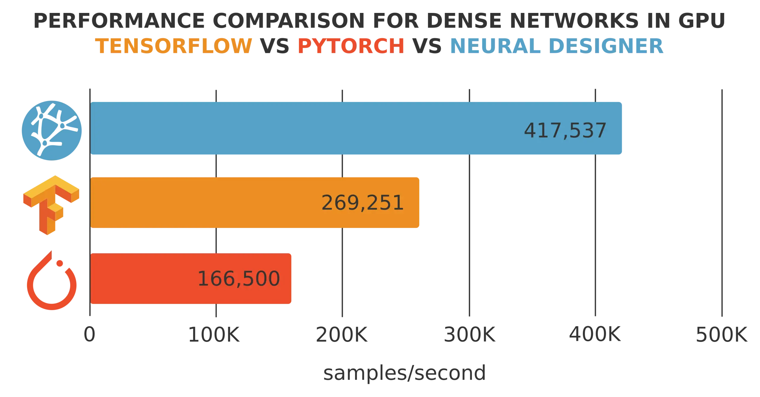
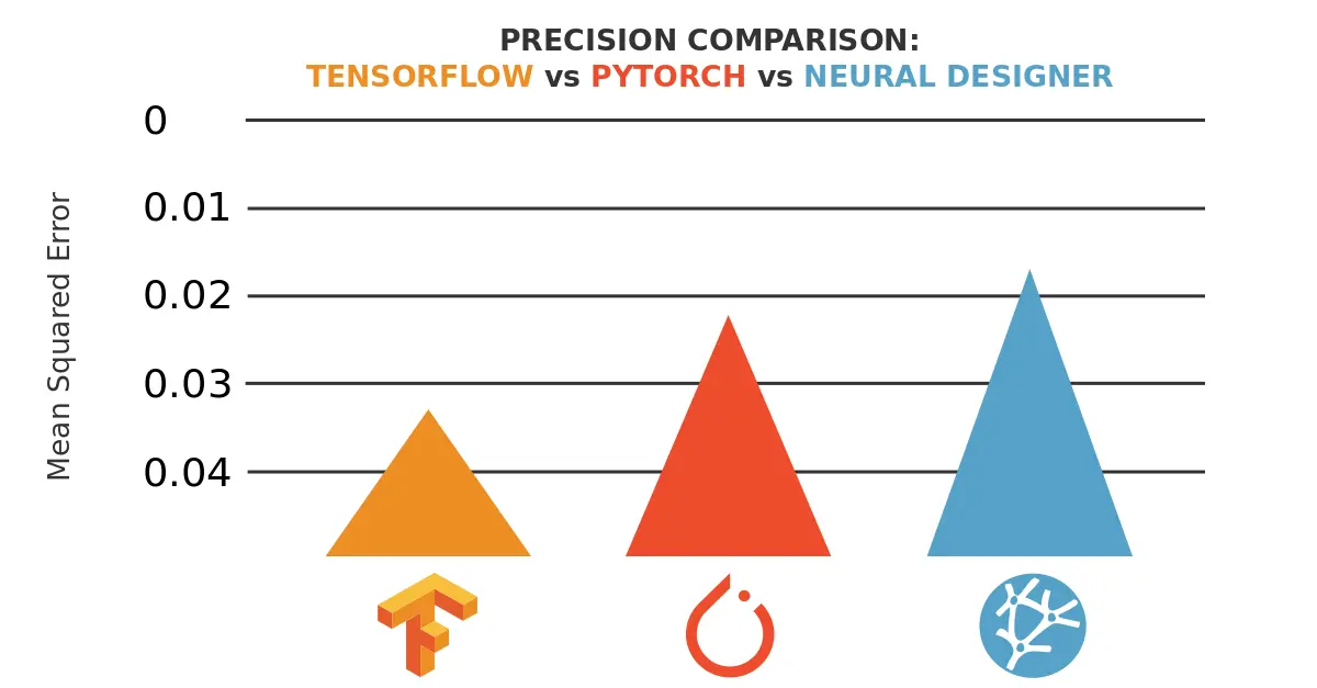
Finally, the following chart depicts the training accuracies of TensorFlow, PyTorch, and Neural Designer for this case graphically.

As we can see, both the minimum and the average mean squared error of Neural Designer using the LM algorithm is smaller than that of TensorFlow and PyTorch using Adam.

Using these metrics, we can say that the precision of Neural Designer for this benchmark is x1.91 times bigger than that of TensorFlow and 1.27 times higher than that of PyTorch.

Regarding the training time, in this benchmark, Neural Designer is about x5.72 times faster than TensorFlow and x8.21 times faster than PyTorch.

Conclusions

Neural Designer implements second-order optimizers, such as the quasi-Newton method and the Levenberg-Marquardt algorithm.
These algorithms have better convergence properties for small and medium-sized datasets than first-order optimizers, such as Adam.

This results in that, for the benchmark described in this post,
the precision of Neural Designer is x1.91 times faster than that of TensorFlow
and x1.27 times faster than that of PyTorch.

To reproduce these results, download the free trial of Neural Designer and follow the steps described in this article.

Precision comparison of machine learning platforms: TensorFlow vs PyTorch vs Neural Designer

Training accuracy comparison of machine learning platforms: TensorFlow vs. PyTorch vs. Neural Designer

Introduction

Benchmark application

Reference computer

Results

Conclusions

Related posts:

Experience the Power of Neural Designer Today

Explanable AI Platform.

Find Us At:

© 2023 - Artificial Intelligence Techniques, Ltd. All rights reserved.