
The volume, variety, and velocity of information stored in security and crime prevention institutions have increased significantly.
The intelligent analysis of all that data can substantially help those security forces adopt these techniques.
This study applies predictive analytics in law enforcement and crime.
Specifically, we develop a neural network to identify patterns of criminal behavior based on location and time variables.
This predictive model will allow security forces to optimize their resources and prevent crimes before they happen.
The developed algorithm can predict crime categories at a given date, time, and district.
Moreover, we can plot the predictions as heat maps, which allows the development of new innovative city systems that could help in the fight against crime.
Contents:
1. Introduction
According to classical theories of criminality, recent literature has focused on the impact of socioeconomic and demographic variables on various types of crime.
To date, the development of efficiency indicators has helped governments improve their efficiency.
Additionally, it has facilitated police work in crime prevention, criminal investigation, apprehension, maintaining order, and providing citizen services.
This work incorporates new methodologies based on machine learning and neural networks into the aforementioned traditional concepts.
These new methods will enhance the allocation of resources to police departments worldwide in their efforts to combat crime.
2. Application type
The variable to be predicted is the number of crimes (a count variable). Therefore, this is an approximation project.
This work aims to demonstrate the ability of neural networks to predict criminal activity in the City and County of San Francisco, based on spatial and temporal variables.
We will explore how a predictive model can enhance the efficiency of a city’s security forces in resource allocation. We also include crime predictions for a given day at different times.
3. Data set
The original dataset contains incidents derived from the San Francisco Police Department’s (SFPD) Crime Incident Reporting System.
The data ranges from 01/01/2003 to 05/13/2015. In particular, it includes 878,049 incident reports with the following variables: day, category, description, weekday, police district, resolution, address, X-coordinate, and Y-coordinate.
The first step is to prepare the data set, which is the source of information for the approximation problem. The original dataset is unsuitable for building a criminality model, so it underwent detailed preprocessing.
We have taken into account two types of variables:
- As inputs, we selected the day, month, day of the week, and time.
- As outputs, we have the number of crimes for every section and police district in four six-hour periods (00:00-6:00, 6:00-12:00, 12:00-18:00, and 18:00-24:00).
The City of San Francisco has ten police districts. The following figure shows this division.

Based on the offenses listed in the San Francisco data set and the ICCS (International Classification of Crime for Statistical Purposes) classification, we conclude that the following types of reports could be grouped in the following sections:
- Section 1: No data available.
- Section 2: Driving under the influence of alcohol, extortion, and kidnapping.
- Section 3: Pornography/obscenity, non-forcible sex offenses, and forcible sex offenses.
- Section 4: Assault, Robbery, and Stolen Property.
- Section 5: Vandalism, burglary, larceny/theft, and vehicle theft.
- Section 6: Drugs/Narcotics and Liquor Laws.
- Section 7: Bad checks, bribery, embezzlement, forgery/counterfeiting, and fraud.
- Section 8: Disorderly conduct, drunkenness, prostitution, gambling, loitering, and runaway.
- Section 9: Weapons law.
- Section 10: Arson.
- Section 11: Fairly offenses, other offenses, and secondary codes.
Neural networks work with numerical values. However, some of the variables in the data set have categorical values.
Therefore, the first step is to assign numerical values to all categorical variables.
- DAY: The day is a numerical value ranging from 1 to 31 for the days in a month.
- MONTH: For the twelve months of the year (from January to December), we have assigned numbers from 1 to 12.
- YEAR: The data we have goes from 2003 to 2015.
Therefore, the year is a numerical value that ranges from 2003 to 2015. - WEEKDAY: For the seven days of the week (from Monday to Sunday), we have assigned numbers from 1 to 7.
- TIME: We divided the 24 hours in a day into four time frames and assigned each time frame a number, as shown in the table below.
| TIME FRAME | NUMBER ASSIGNED |
|---|---|
| 00:00-6:00 | 1 |
| 6:00-12:00 | 2 |
| 12:00-18:00 | 3 |
| 18:00-24:00 | 4 |
- NUMBER OF CRIMES PER POLICE DISTRICT: We want to predict this variable. As shown in the figure of the distribution of police departments in the city of San Francisco, there are ten police districts in San Francisco:
Bayview, Central, Ingleside, Mission, Northern, Park, Richmond, Southern, Taraval, and Tenderloin.
The data set contains information about the number of crimes committed at a given time in one of these districts. This variable is numerical, so it doesn’t require any changes.
The variables are of two types:
- Input variables: these are the predictors of the criminality model (day, month, year, weekday, and time).
- Target variables: These are the variables to be predicted, specifically the crime count per police department within a given time frame for each section.
On the other hand, cases can be of three types:
- Training cases are used to build different criminality models with different topologies.
- Selection cases are used to select the criminality model with the best predictive capabilities.
- Test cases are used to validate the performance of the criminality model.
The following pie chart illustrates the uses of all cases in the dataset.
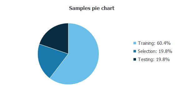
The data is divided into training, selection, and testing subsets, comprising 60%, 20%, and 20% of the instances.
This results in 11,302 cases for training, 3,676 for selection, and 3,676 for testing for each section.
Statistics
Basic statistics are valuable information when designing a model, as they provide important insights into our application.
The total number of crimes in the data set is 674,656. They comprise the period from January 1, 2003, to May 13, 2015.
Therefore, the average number of crimes per day is 149.59. The following table shows that Richmond has the lowest number of offenses, while Southern has the highest.
| Count | Crimes/day | |
|---|---|---|
| Bayview | 72560 | 16.088 |
| Central | 69252 | 15.355 |
| Ingleside | 65140 | 14.443 |
| Mission | 96218 | 21.334 |
| Northern | 87380 | 19.374 |
| Park | 37930 | 8.410 |
| Richmond | 36860 | 8.172 |
| Southern | 118323 | 26.235 |
| Taraval | 52963 | 11.743 |
| Tenderloin | 64829 | 14.374 |
The most common crime types are those belonging to Section 5 (vandalism, burglary, larceny/theft, and vehicle theft), totaling 310,160 offenses.
On the other hand, Section 10 (arson) has the lowest rate, with a total of 1,513 crimes reported. The following table shows those statistics:
| Count | Crimes/day | |
|---|---|---|
| Section 2 | 4865 | 1.078 |
| Section 3 | 4558 | 1.010 |
| Section 4 | 104415 | 23.151 |
| Section 5 | 310160 | 68.771 |
| Section 6 | 55874 | 12.388 |
| Section 7 | 29149 | 6.463 |
| Section 8 | 19401 | 4.301 |
| Section 9 | 8555 | 1.896 |
| Section 10 | 1513 | 0.335 |
| Section 11 | 136167 | 30.192 |
Finally, if we calculate the statistics by type of crime and location, the combination of Southern and Section 5 has the highest number of crimes (57,961).
On the other hand, the combination of Tenderloin and Section 10 has the lowest number (60). The following table shows all of the above.
| Section 2 | Section 3 | Section 4 | Section 5 | Section 6 | Section 7 | Section 8 | Section 9 | Section 10 | Section 11 | |
|---|---|---|---|---|---|---|---|---|---|---|
| Bayview | 505 | 411 | 12969 | 26623 | 4612 | 1830 | 876 | 1647 | 393 | 18715 |
| Central | 408 | 403 | 9486 | 38258 | 1946 | 3745 | 1933 | 487 | 111 | 9605 |
| Ingleside | 583 | 526 | 11668 | 27901 | 2479 | 2353 | 577 | 1130 | 182 | 14503 |
| Mission | 695 | 756 | 15408 | 34410 | 9252 | 3487 | 6017 | 1329 | 145 | 20769 |
| Northern | 515 | 449 | 11658 | 46179 | 4635 | 3550 | 2942 | 789 | 149 | 13232 |
| Park | 278 | 218 | 4647 | 18610 | 2722 | 1564 | 1159 | 357 | 65 | 6628 |
| Richmond | 446 | 227 | 4195 | 19886 | 1080 | 1838 | 387 | 327 | 103 | 6157 |
| Southern | 684 | 840 | 17068 | 57961 | 9613 | 6172 | 2159 | 1128 | 185 | 22513 |
| Taraval | 429 | 402 | 7099 | 26319 | 1653 | 2793 | 953 | 567 | 120 | 9597 |
| Tenderloin | 322 | 326 | 10217 | 14013 | 17882 | 1817 | 2398 | 794 | 60 | 14447 |
The data set used to design the approximation model that predicts city crime contains the number of crimes for all sections and districts over a 4-hour period.
For each section, we have a dataset of 18,385 instances and 15 variables (day, month, year, weekday, time, and the number of crimes for the police districts: Bayview, Central, Ingleside, Mission, Northern, Park, Richmond, Southern, Taraval, and Tenderloin). The total number of data is 275,775.
The table below shows the minimums, maximums, means, and standard deviations of the data corresponding to Section 5 crimes (burglary, larceny/theft, vandalism, and vehicle theft).
As we can see, the district with the most crimes is the Southern.
| Minimum | Maximum | Mean | Deviation | |
|---|---|---|---|---|
| Day | 1 | 31 | ||
| Month | 1 | 12 | ||
| Year | 2003 | 2015 | ||
| Weekday | 1 | 7 | ||
| Time | 1 | 4 | ||
| Bayview | 0 | 19 | 2.960 | 1.644 |
| Central | 0 | 22 | 4.254 | 2.121 |
| Ingleside | 0 | 20 | 3.102 | 1.725 |
| Mission | 0 | 22 | 3.826 | 1.992 |
| Northern | 0 | 30 | 5.135 | 2.555 |
| Park | 0 | 17 | 2.069 | 1.326 |
| Richmond | 0 | 16 | 2.211 | 1.413 |
| Southern | 0 | 38 | 6.445 | 3.095 |
| Taraval | 0 | 20 | 2.926 | 1.662 |
| Tenderloin | 0 | 15 | 1.558 | 1.089 |
Histograms show the distribution of the data over its entire range. For example, the following figure is a histogram of Section 5 crimes in Southern.

This histogram has a normal distribution centered on 5.7 crimes per 4 hours.
4. Neural network
A neural network is a computational model inspired by the brain and built from interconnected artificial neurons.
Its main strength is learning to perform tasks such as pattern recognition, relationship discovery, and trend forecasting.
No more hidden layers are needed, for this is a class of universal approximators.
For each section, the neural network has five inputs (day, month, year, weekday, and time) and ten output neurons (the number of crimes in that period for each district).

5. Training strategy
While the problem constrains the number of input and output neurons, the number of hidden neurons is a design variable that can be adjusted. Therefore, we conducted a detailed analysis of order selection to determine the optimal network architecture.
The loss index chosen for this application is the normalized squared error between the neural network’s outputs and the dataset’s targets.
This error is a very standard loss index in data modeling. A regularization term is added to the loss expression to obtain smooth solutions.
The selected training algorithm for solving the problem is a quasi-Newton method with BFGS training direction and Brent optimal training rate. This training algorithm is a standard method that performs well for both small and large problems.
6. Testing analysis
We calculated the errors between the neural network outputs and their corresponding targets in the testing set to test the model’s predictive capabilities.
The following table presents the results obtained from this testing analysis for each district.
| Mean error (%) | |
|---|---|
| Bayview | 8.902 |
| Central | 7.818 |
| Ingleside | 7.966 |
| Mission | 8.371 |
| Northern | 6.862 |
| Park | 9.382 |
| Richmond | 8.946 |
| Southern | 6.041 |
| Taraval | 7.394 |
| Tenderloin | 7.875 |
Here, the mean errors lie in the range of 5-10%, which are good numbers for this kind of problem.
From the table above, we can see that the neural network predicts crime rates with reasonable accuracy.
The neural network is now ready to move to the production phase.
7. Model deployment
The following figure shows the crime predictions for Section 5 on Thanksgiving Day (Thursday, November 23rd) from 00:00 to 06:00.

As can be seen, most districts have low rates, but Southern has a medium rate.
Similarly, the following figure shows the exact predictions for the 06:00-12:00 period.

The increase continues, with Southern, Northern, and Central showing the highest crime levels, while Tenderloin shows the lowest, and the rest of the districts fall in between.
As the day progresses, between 12:00 and 18:00, the Southern District will reach a high worrying ratio. The Central and Northern districts will also be at risk. The Tenderloin, Richmond, and Park districts will no longer be as secure as earlier, and the Bayview, Ingleside, Mission, and Taraval districts will be at intermediate risk.

The highest ratios will occur late evening (18:00-24:00), especially in Southern, Central, and Northern districts. The ratios will be intermediate in Bayview, Ingleside, Mission, and Taraval districts (also in Tenderloin). On the other hand, the districts of Richmond and Park will present the lowest ratios.

We can also examine how crimes will evolve. For example, the following figure shows the evolution of Section 5 offenses in Southern during a whole week and from 12:00 to 18:00.

As we can see, the number of crimes increases throughout the week, from Sunday to Saturday.
Conclusions
In this study, we have utilized machine learning based on neural networks to support the police forces of the City and County of San Francisco.
Like many others globally, this city is increasing the volume, variety, and velocity of information stored about crimes.
By recognizing patterns of criminal behavior based on temporal and spatial variables, we have designed a predictive model to optimize police resources and prevent crimes before they occur.
- We have observed how Section 5 crimes in the Southern District represent the darkest points of criminality in the City of San Francisco.
- Section 10 crimes in the Tenderloin District have the smallest number of crimes in that city.
- The predictive model indicates that Section 5 crimes increase as the day progresses, with the 18:00-24:00 period being the most dangerous, particularly in the Southern, Central, and Northern Districts.
- Conversely, the lowest ratios for that section occur in the 00:00-06:00 period in the Tenderloin district.
Due to the crime maps and evolution graphs generated as examples, we can observe clusters of crime areas and periods.
This enables the police to allocate resources effectively, preventing crimes and reducing the risk to citizens.
The study presented in this chapter leads us to conclude that neural networks have an excellent capacity for crime prevention.
Implementing these systems in the SFPD will enable better allocation of human resources. That will result in greater efficiency of those police forces.
At the same time, these advanced analytics methods enhance existing ones that leverage traditional socioeconomic and demographic variables, often utilizing Data Envelopment Analysis as an optimization technique for inputs/outputs.
References:
- The data set used in this study contains incidents reported by the San Francisco Police Department (SFPD) and is published by San Francisco Open Data, the central clearinghouse for data published by the City and County of San Francisco.
- The International Classification of Crime for Statistical Purposes (ICCS).