
Deployment in machine learning is the process of applying a model to make predictions on new data.
It involves organizing and presenting the learned knowledge so that it can be used effectively by the customer.
Depending on the needs, deployment can be as simple as producing a report or as advanced as setting up a continuous learning system.
You can use the following techniques for deploying a neural network:
- 7.1. Neural network outputs
- 7.2. Output data
- 7.3. Directional outputs
- 7.4. Mathematical expression
- 7.5. Python expression
- 7.6. C++ expression
7.1. Neural network outputs
A neural network produces a set of outputs for each set of inputs applied.
The table below shows input attributes and their corresponding outputs when estimating a car’s fuel consumption.
| Cylinders | Displacement | Horsepower | Weight | Acceleration | Model year | Fuel consumption |
|---|---|---|---|---|---|---|
| 8 | 307 | 130 | 3504 | 12 | 1980 | 17 mpg |
7.2. Output data
Often, the goal is to predict outputs for multiple cases stored in a data file, where each row contains the input values.
The model then produces a new file with the corresponding outputs.
The table below shows how a neural network estimates conversion probabilities for customers in a marketing campaign based on engagement factors.
| Recency | Frequency | Monetary | Conversion |
|---|---|---|---|
| 2 months | 5 times | 125 USD | 70% |
| 5 months | 2 times | 20 USD | 8% |
| 3 months | 9 times | 225 USD | 85% |
| 4 months | 1 time | 15 USD | 5% |
| 1 months | 3 times | 70 USD | 75% |
7.3. Directional outputs
By varying one input while keeping the others fixed, we can see how that factor influences the model’s output.
These directional outputs are helpful not only for understanding the model but also for improving designs or processes.
The following table shows the reference point for plotting all the directional output charts. In this case, the model estimates the residuary resistance of a sailing yacht as a function of design parameters and sailing conditions.
| Center of buoyancy | -2.38 |
| Prismatic coefficient | 0.56 |
| length displacement | 4.79 |
| Beam draught ratio | 3.94 |
| length beam ratio | 3.21 |
The following chart shows how the residuary resistance varies with the Froude number (which represents the velocity of the yacht), with all the other inputs being fixed.
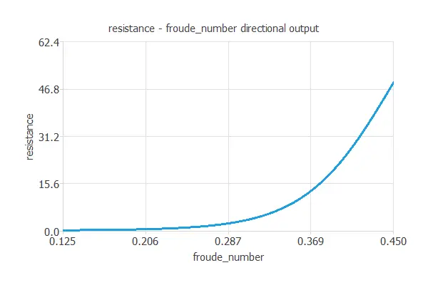
As we can see, the residuary resistance increases exponentially for high values of the Froude number. Therefore, this yacht design does not perform well at high speeds.
7.4. Mathematical expression
Next, we list an example of the mathematical model represented by a neural network.
scaled_shear_rate = 2*(shear_rate-50)/(90-50)-1;
scaled_particle_diameter = 2*(particle_diameter-0.72)/(6.596-0.72)-1;
y_1_1 = tanh(-1.06007+(scaled_shear_rate*0.448487)+(scaled_particle_diameter*-0.861393));
y_1_2 = tanh(0.756922+(scaled_shear_rate*2.00716)+(scaled_particle_diameter*0.391539));
y_1_3 = tanh(0.862072+(scaled_shear_rate*-0.726115)+(scaled_particle_diameter*-1.46053));
scaled_particles_adhering = (-1.30536+(y_1_1*-1.0244)+(y_1_2*0.56055)+(y_1_3*-0.565459));
particles_adhering = (0.5*(scaled_particles_adhering+1.0)*(74.75-13.22)+13.22);
You can easily embed the above code into any application that uses the model.
For that, you only need to adapt the mathematical expression to the syntax of your programming language.
7.5. Python expression
We can export the mathematical expression the model represents to different programming languages, such as Python.
The following example is a neural network implemented in the Python programming language.
def expression(inputs) :
if type(inputs) != list:
print('Argument must be a list')
return
if len(inputs) != 4:
print('Incorrect number of inputs')
return
temperature=inputs[0]
exhaustt_vacuum=inputs[1]
ambient_pressure=inputs[2]
relative_humidity=inputs[3]
scaled_temperature = (temperature-19.6512)/7.45247
scaled_exhaustt_vacuum = 2*(exhaustt_vacuum-25.36)/(81.56-25.36)-1
scaled_ambient_pressure = (ambient_pressure-1013.26)/5.93878
scaled_relative_humidity = (relative_humidity-73.309)/14.6003
		y_1_1 = tanh (-0.155062+ (scaled_temperature*0.203034)+ (scaled_exhaustt_vacuum*0.731056)+ (scaled_ambient_pressure*-0.191671)+ (scaled_relative_humidity*0.0158643))
		y_1_2 = tanh (-0.29098+ (scaled_temperature*-0.023069)+ (scaled_exhaustt_vacuum*-0.263476)+ (scaled_ambient_pressure*-0.231774)+ (scaled_relative_humidity*0.333626))
		y_1_3 = tanh (0.570558+ (scaled_temperature*0.573079)+ (scaled_exhaustt_vacuum*-0.0279703)+ (scaled_ambient_pressure*0.111165)+ (scaled_relative_humidity*0.00867248))
		scaled_energy_output =  (0.15981+ (y_1_1*-0.383639)+ (y_1_2*-0.126028)+ (y_1_3*-0.745885))
energy_output = (0.5*(scaled_energy_output+1.0)*(495.76-420.26)+420.26)
		return energy_output
You can easily integrate this code into any Python application that uses the model.
7.6. C++ expression
C++ is one of the most widely used programming languages.
The following code is an example of a neural network in the C programming language.
#include
using namespace std;
vector scaling_layer(const vector& inputs)
{
vector outputs(5);
outputs[0] = inputs[0]*0.3025558293-1;
outputs[1] = inputs[1]*0.3025558293-1;
outputs[2] = inputs[2]*0.4306863844-0.1386272311;
outputs[3] = inputs[3]*5.421008924e-20-1;
outputs[4] = inputs[4]*5.421008924e-20+1;
return outputs;
}
vector perceptron_layer_0(const vector& inputs)
{
vector combinations(3);
combinations[0] = 0.02009 -0.880635*inputs[0] +0.815813*inputs[1] -0.106329*inputs[2] -0.117222*inputs[3] -0.210783*inputs[4];
combinations[1] = 0.0355442 -0.0121058*inputs[0] +0.0725463*inputs[1] +0.0671187*inputs[2] -0.0893239*inputs[3] +0.205473*inputs[4];
combinations[2] = -0.00834767 +0.0153575*inputs[0] -0.00712658*inputs[1] +0.0125823*inputs[2] -0.0126559*inputs[3] -0.0117719*inputs[4];
vector activations(3);
activations[0] = tanh(combinations[0]);
activations[1] = tanh(combinations[1]);
activations[2] = tanh(combinations[2]);
return activations;
}
vector perceptron_layer_1(const vector& inputs)
{
vector combinations(1);
combinations[0] = -0.044036 +1.01136*inputs[0] -0.244702*inputs[1] +0.00911695*inputs[2];
vector activations(1);
activations[0] = combinations[0];
return activations;
}
vector unscaling_layer(const vector& inputs)
{
vector outputs(1);
outputs[0] = inputs[0]*0.7265999913+0.7265999913;
return outputs;
}
vector bounding_layer(const vector& inputs)
{
vector outputs(1);
outputs[0] = inputs[0];
return outputs;
}
vector neural_network(const vector& inputs)
{
vector outputs;
outputs = scaling_layer(inputs);
outputs = perceptron_layer_0(outputs);
outputs = perceptron_layer_1(outputs);
outputs = unscaling_layer(outputs);
outputs = bounding_layer(outputs);
return outputs;
}
int main(){return 0;}
You can easily embed the above code into any C++ application that uses the model.
Bibliography ⇒