A machine learning dataset collects data to create and train an approximation, classification, or forecasting model. Central to this process is the data source, the specific origin point of the data being utilized. These data sources come in various formats, such as Excel files, .csv files, databases, image data, and more.
Before building a model, it is necessary to transform the data into numbers; this involves collecting the data in a matrix of real numbers, thereby creating the data matrix. Each column symbolizes a specific variable within a dataset, while each row corresponds to an individual sample within the dataset.
A variable encompasses any measurable or countable characteristic, number, or quantity. It serves as an attribute that describes a person, place, thing, or concept.
The variable’s value can “vary” from one entity to another. According to their type, we can consider different types of variables: numeric, ordinal, binary, or categorical variables.
Variables can be used as inputs or targets. Input variables are the independent variables in the model (they are also called features or attributes), and target variables are the dependent variables in the model.
A sample represents an observation encompassing all variables within a dataset. Additionally, these samples serve various purposes, prompting their division into three distinct subsets. These are the training set (used to build different candidate models), the selection set (used to select the model that exhibits the best properties), and the test set (used to validate the final model).
Sometimes, the dataset may be incomplete or have missing values. This is one of the main problems when applying neural networks to real-world problems. We can unuse the whole sample or impute such a value to solve it.
Contents
1. Data matrix
Before building a model, we need to collect the data in a matrix of real numbers.
Let denote ( p) the number of rows and $q$ the number of columns.
It is a matrix $d in {R}^{p times q}$.
As we can see, machine learning models require all data to be real numbers.
The data matrix has the following form,
begin{eqnarray}
d = left(
begin{array}{ccc}
d_{1,1} & cdots & d_{1,q}\
vdots & ddots & vdots \
d_{p,1} & cdots & d_{p,q}\
end{array}
right).
end{eqnarray}
Samples
A sample is a vector $u in {R}^{p}$, where $p$ is the number of rows in the data matrix.
In this regard, the data matrix contains $q$ variables,
begin{eqnarray}
u_{i}:=col_{i}(d), quad i=1,ldots,q.
end{eqnarray}
The samples will also have different uses. We divide the samples into three different subsets. These are the training set (used to build different candidate models), the selection set (used to select the model that exhibits the best properties), and the test set (used to validate the final model).
Variables
A variable is a vector $v in {R}^{q}$, where $q$ is the number of columns in the data matrix.
In this regard, the data matrix contains $p$ samples,
begin{eqnarray}
v_{i}:=row_{i}(d), quad i=1,ldots,p.
end{eqnarray}
The variable’s value can “vary” from one entity to another. According to their type, we can consider different types of variables: numeric, ordinal, binary, or categorical variables.
Variables can be used as inputs or targets. Input variables are the independent variables in the model (they are also called features or attributes), and target variables are the dependent variables in the model.
Our source of information may not be in a direct matrix format.
For example, the information may be distributed in several tables of a database.
We can also find sets of images to, for example, diagnose a tumor.
In addition, some data may not be real numbers.
For example, a customer’s country (Spain, France, etc.) is categorical.
This means that an essential part of building machine learning models is the creation of a data matrix with the correct format.
The following example from the industry sector shows a data matrix of a real model: Wind turbine data matrix
A wind turbine manufacturer wants to know the electrical power generated by the device at different wind speeds.
To do this, they measure different operating scenarios and generate the following data matrix,
begin{eqnarray}nonumber
d = left(
begin{array}{cc}
380.048 & 5.311\
453.769 & 5.672\
vdots & vdots \
2820.466 & 9.973\
end{array}
right).
end{eqnarray}
The number of columns in the data matrix is $q=2$, a simple matrix.
Each column corresponds to a variable.
In this case, we have the wind speed (in meters per second) and the corresponding power generated by the turbine (in kilowatts).
The first column is the input, and the second column is the target.
The number of rows in the data matrix is $p=48007$.
Each row corresponds to a sample.
Each sample contains values of the two variables.
2. Data analysis
Before building a model, we need to analyze the data statistically to understand what it represents.
Statistics
The most basic analysis involves examining the statistics for each variable, with the most important statistical parameters being the minimum, maximum, mean, and standard deviation.
Distributions
Another descriptive analysis is that of the distributions of each variable.
For the predictive model to be of higher quality, we must check that all the variables in a dataset have a uniform or normal distribution.
We can calculate different types of distributions, such as histograms, pie charts, medians, quartiles, or box plots.
Correlations
We can also discover dependencies between the variables of the dataset from the correlations.
A correlation is a numerical value between -1 and 1 that expresses the strength of the relationship between two variables.
When the correlation approaches 1 between two variables, they are positively related. Conversely, a correlation near 0 suggests no discernible relationship between the study variables. In contrast, if the correlation approaches -1, the variables are negatively related.
Outliers
We can also analyze the data to detect potential problems. One of the most common problems is outliers.
Outliers, which are abnormal observations in the data, have the potential to disrupt and confound the training process.
To address these outliers, we can employ Tukey’s univariate test or utilize the Local Outlier Factor, a multivariate method.
Filtering
We can also filter the data to create models with subsets of it. Filtering is usually temporary; we keep the entire data set, but only a part is used for the calculation.
Filtering requires that you specify a rule or logic to identify the cases you want to include in the analysis.
Scaling
On the other hand, you should always scale the variables before training a neural network.
Scaling puts the data into a suitable range for computation, usually done variable by variable, since each can have different ranges.
Some of the most common methods are minimum–maximum, mean–standard deviation, and logarithmic scaling.
Batching
Training algorithms for neural networks do not work with the data matrix directly. Instead, they use data structures called data batches.
A batch of data contains two tensors, one with input data and one with target data, and the range of these batches depends on the model type.
Conclusions
Datasets collect the data needed to create and train a model. In general, the data must be transformed to adapt it to machine learning and generate the data matrix.
Subsequently, it is advisable to perform a statistical study of the data to deal with potential problems such as outliers.