\begin{eqnarray}v_{j} := column_{j}(d), \quad j=1,\ldots,q\quad\end{eqnarray}
and the samples
\begin{eqnarray}u_{i} := column_{i}(d), \quad i=1,\ldots,p\quad\end{eqnarray}
(columns and rows of the data set).
The values that a variable takes for each sample in the data set are
\begin{eqnarray}\quad v_j=(d_{1j}, \ldots, d_{pj}), \quad j=1,\ldots,q.\end{eqnarray}
Contents
2. Minimum and maximum
The minimum of a variable is the smallest value of that variable in the data set.
The minimum of the variable is denoted by $v_{jmin}$, and it is defined as follows,
\begin{eqnarray}
\boxed{
v_{jmin} = \min_{i = 1, \ldots, p} d_{ij}.
}
\end{eqnarray}
A variable’s maximum is the variable’s biggest value in the data set.
Similarly, the maximum is denoted by $v_{jmax}$, and it is defined as follows,
\begin{eqnarray}
\boxed{
v_{jmax} = \max_{i=1, \ldots, p} d_{ij}.
}
\end{eqnarray}
3. Mean and standard deviation
The mean of a variable is the average value of that variable in the data set. The mean is denoted by $v_{jmean}$ and is defined as,
\begin{eqnarray}
\boxed{v_{jmean} = \frac{1}{p}\sum_{i=1}^{p} d_{ij}.}
\end{eqnarray}
where $d_{ij}$ is the data matrix element and $p$ is the number of samples.
The standard deviation measures how dispersed the data is about the mean. The standard deviation of a variable is denoted by $v_{jstd}$ and is defined as,
\begin{eqnarray}
\boxed{
v_{jstd} = \sqrt{\frac{1}{p}\sum_{i=1}^{p}\left(d_{ij}-v_{jmean}\right)^2}.
}
\end{eqnarray}
where $v_{jmean}$ is the mean of the variable $v_{j}$.
The graphical representation is the standard distribution curve, called the Gaussian bell.
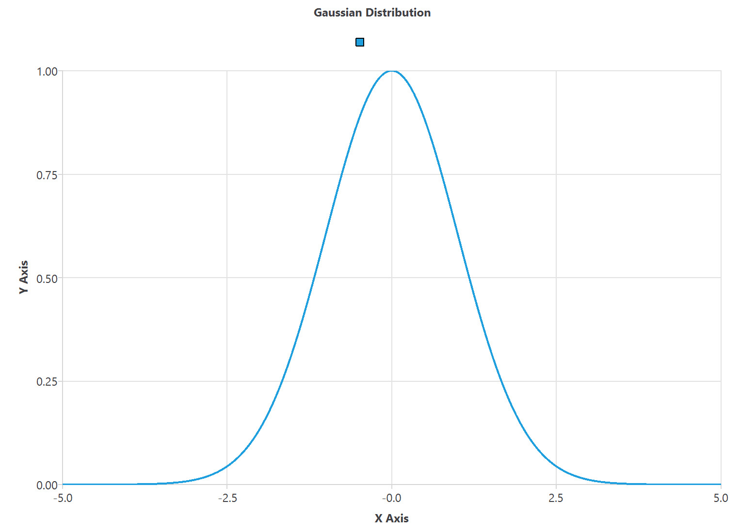
A low standard deviation means that all the values are close to the mean.
Conversely, a high standard deviation means the values are spread out around the mean and from each other.
Example: Predict the noise generated by airfoil blades
NASA conducts a study of the noise generated by an aircraft in order to make a model to reduce it.
The file airfoil_self_noise.cvs contains the data for this example.
Here the number of variables (columns) is 6, and the number of instances (rows) is 1503.
We can calculate the basic statistics of each variable using the formulas described above.
The following table displays the minimum, maximum, mean, and standard deviation for every input variable in the data set.
| Name | Minimum | Maximum | Mean | Deviation |
| frequency | 200 | 20000 | 2890 | 3150 |
| angle_of_attack | 0 | 0.22 | 6.78 | 5.92 |
| chord_length | 0.0254 | 0.305 | 0.137 | 0.0935 |
| free_stream_velocity | 31.7 | 71.3 | 50.9 | 15.6 |
| suction_side_displacement_thickness | 0.000401 | 0.0584 | 0.0111 | 0.0132 |
| scaled_sound_pressure_level | 103 | 141 | 125 | 6.9 |
By performing this simple statistical analysis, we can check the consistency of the data.
4. Conclusions
Statistics put the data set in context.
It is essential to perform a simple statistical analysis to check the consistency of the data before building the model.
This is done by calculating each variable’s most important statistical parameters, such as the minimum and maximum values, mean, and standard deviation.