Text classification is a machine learning technique that assigns predefined categories to free-form text.
With text classifiers, you can organize and categorize almost any kind of text, from documents and medical studies to extensive archives or even the entire web.
In this post, we explain this text mining technique along with its main stages and procedures.
Contents
Introduction
The categorization or classification of information is one of the most widely used branches of Text Mining.
The premise of classification techniques is straightforward: starting from a set of data with an assigned category or label, the objective is to build a system that identifies patterns in existing documents to determine their class.
Text classification uses labeled documents to train a system that learns patterns and assigns each document to one of the predefined classes.
Depending on the number of classes, text classification problems can be binary or multiple.
In binary classification, the model determines whether a document belongs to a specific class—for example, spam detection, where an email is classified as either spam or not.
In multiple classification, each document is assigned to one class from several options—for instance, sentiment analysis, where the categories can be happiness, sadness, joy, and others.
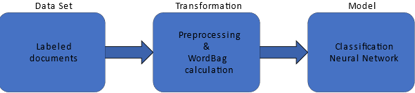 We can divide the text classification process into the following steps:
- Data processing and transformation
- Model training
- Testing analysis
1. Data processing and transformation
The transformation process in a classification problem comprises two stages: normalization and numerical representation.
Normalization
Sometimes, in classification problems, the computational cost is very high, and reducing the number of input variables helps obtain better results faster.
For this purpose, document normalization is generally applied. This process consists of using some of the following techniques for reducing the number of input words:
- Lowercase transformation: for example, “LoWerCaSE” is transformed into “lowercase.”
- Punctuation signs and special characters removal: punctuation signs and special characters like “;”,” #”, or “=” are removed.
- Stop words elimination: Stop words are commonly used words in any language that don’t provide any information for our model. For example, some stop words in the English language are “myself”, “can”, and “under”.
- Short and long word deletion: short words are eliminated because they do not provide much information, for example, the word “he”. On the other hand, long words are eliminated because of their low frequency in the documents.
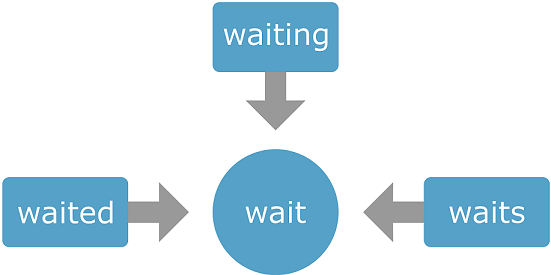

- Stemming: Every word is composed of a root, a lemma (or lexeme), the part of the word that does not vary and indicates its central meaning, and a morpheme, particles that are added to the root to form new words.
The stemming technique replaces each word with its lemma to obtain fewer input words.
Once we have processed and normalized the documents, we must transform them into a numerical format that neural networks can process.
Numerical representation
The intuition behind this idea lies in representing documents as vectors in an n-dimensional vector space.
Therefore, the neural network can interpret and utilize these vectors to perform various tasks.
Among the simplest traditional text representation techniques is a Bag of Words.
Bag of Words
Bag-of-Words (BoW) consists of constructing a dictionary for the working dataset and representing each document as a count of the words in it.
This type of representation represents the document as a vector with a length equal to the number of words in the dictionary.
Each vector element denotes the frequency of each token’s usage in the document.
| water | steak | want | don’t | the | some | and | I | |
|---|---|---|---|---|---|---|---|---|
| “I want some water.” | 1 | 0 | 1 | 0 | 0 | 1 | 0 | 1 |
| “I want the steak.” | 0 | 1 | 1 | 0 | 1 | 0 | 0 | 1 |
| “I want steak, and I want water.” | 1 | 1 | 1 | 0 | 0 | 0 | 1 | 1 |
| “I don’t want water.” | 1 | 0 | 1 | 1 | 0 | 0 | 0 | 1 |
We refer to this method as a “bag of words” since it does not preserve the order of the words.
It is also important to note that if new documents are introduced with vocabulary not present in the existing corpus, they can be transformed by omitting the unknown words.
The BoW model has several drawbacks in its use.
One of the most relevant is that when the corpus size is considerable, the vocabulary size is consequently increased.
Therefore, very sparse vector sets are obtained, with many zeros and large sizes, which implies a higher memory consumption.
2. Model training
Once the document’s numerical representation has been obtained, we can start model training using a classification neural network.
A classification neural network usually requires a scaling layer, one or several perceptron layers, and a probabilistic layer.
3. Testing analysis
As with any classification problem, model evaluation is essential.
However, in text classification problems, evaluation measures are not absolute, as they depend on the specific classification task: classifying medical texts is not the same as classifying whether a review is positive or negative.
Therefore, the most common approach is to consult the literature for baselines for similar tasks and compare them to determine if we are achieving acceptable results.
As with a traditional classification task, the most used metrics are:
Confusion matrix
In the confusion matrix, the rows represent the target classes in the data set, and the columns represent the predicted output classes from the neural network.
The following table represents the confusion matrix:
| Predict class 1 | … | Predict class N | |
|---|---|---|---|
| Red class 1 | # | # | # |
| … | # | # | # |
| Red class N | # | # | # |
- Accuracy: The proportion of correctly classified documents from the total for which the model predicted the class c.
div style=”max-width: 100%; overflow-x:auto”>
$$ precision = frac{# true positives}{# true positives + # false positives}$$ - Recall: The proportion of correctly classified documents among all documents in the training set with class c.
$$ recall = frac{# true positives}{# true positives + # false negatives}$$ - F1-Score: Generally, a good classifier should balance accuracy and recall. For this purpose, we use the F1-score metric, which considers both parameters. This score will penalize the total value if either of the two values is too low.
$$ F1 = frac{2·precision·recall}{precision + recal}$$
Additionally, we must strike a balance between overfitting and underfitting to achieve a high-quality classifier.
An underfitted model has low variance, meaning that when the same data is introduced, the exact prediction is obtained; however, this prediction is too far from reality.
This phenomenon occurs when the model has insufficient training data to find the existing patterns in the data.
Alternatively, achieving the optimal operational point involves evaluating the model with entirely new, untrained data.
For this reason, it is advisable to subdivide the corpus into multiple subsets (training, testing, and selection).
Conclusions
Text classification is one of the most widely used techniques in machine learning.
It can be applied to tasks such as sentiment analysis of reviews or prioritizing support messages by urgency.
This article reviews the key stages of a text classification project, including data processing and transformation, model training, and testing analysis.
By following these steps, you can build accurate and effective text classification models.