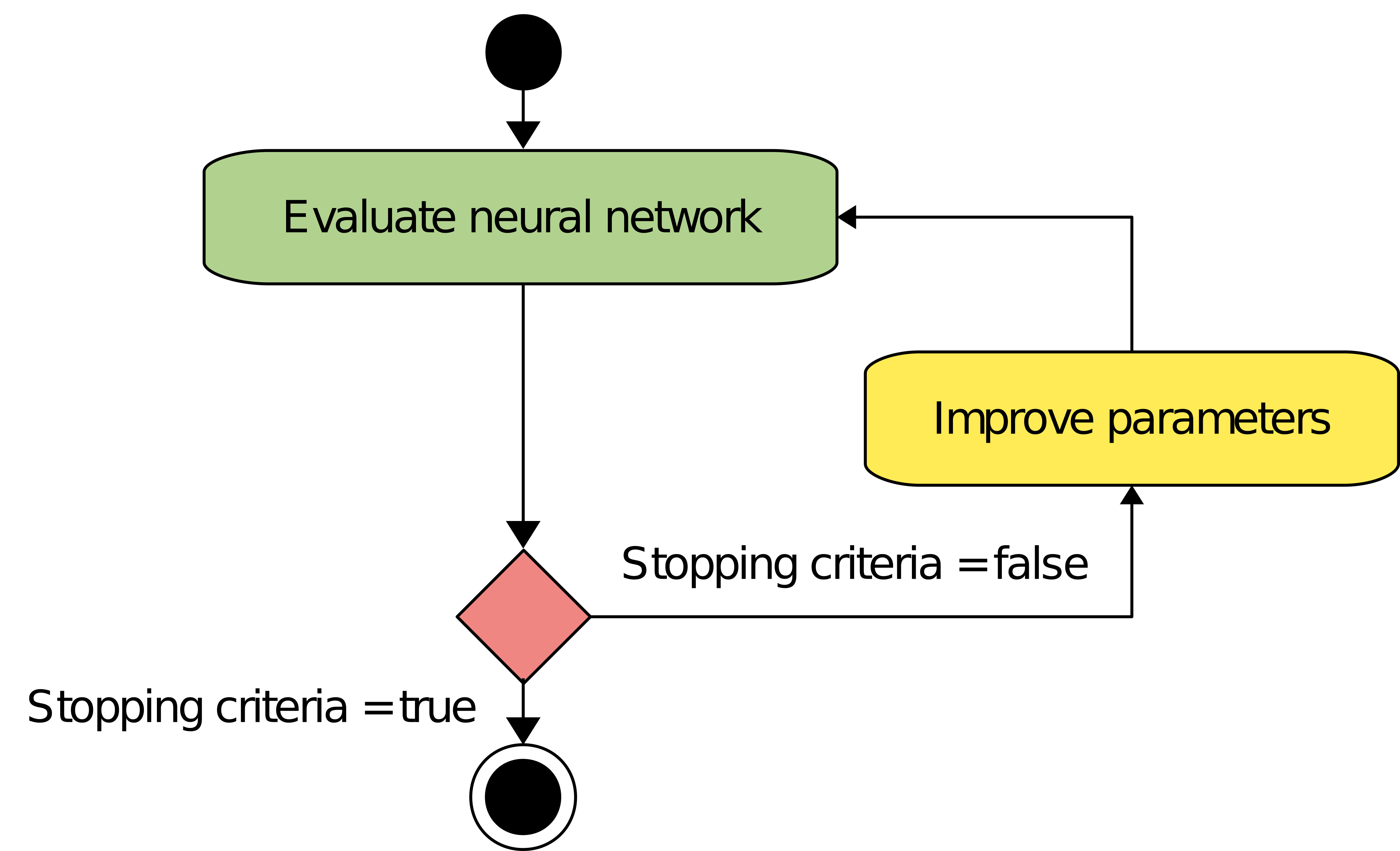
An optimizer is the procedure that updates a neural network’s trainable parameters to reduce its loss. It is one part of the training strategy, together with the loss function, data batches, learning-rate schedule, regularization, and stopping criteria.
There is no optimizer that is best for every neural network. Full-batch methods can exploit accurate gradient and curvature information on modest problems, while mini-batch methods make it possible to train networks with large datasets and millions or billions of parameters.
This guide explains the main optimizer families, from gradient descent and curvature-aware methods to stochastic gradient descent, Adam, and AdamW. It compares their memory requirements, batch regimes, strengths, and limitations so that you can select an appropriate method for your problem.
- The optimization problem
- Full-batch and mini-batch training
- Gradient descent
- Newton’s method
- Quasi-Newton: BFGS and L-BFGS
- Levenberg-Marquardt
- Stochastic gradient descent
- Adam and AdamW
- Optimizer comparison
- How to choose an optimizer
- Emerging optimizers
- Conclusions
The optimization problem
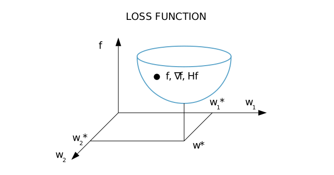
Training searches for a parameter vector \(\boldsymbol{\theta}^{*}\) that minimizes a loss function. For a batch of \(B\) samples, a common formulation is
where \(\ell_b\) is the error for sample \(b\), \(\Omega\) is an optional regularization term, and \(\lambda\) controls its contribution. Backpropagation computes the gradient
which indicates how the loss changes with each parameter. Curvature-aware methods also use the Hessian \(\mathbf{H}=\nabla^2 f\), an approximation to it, or a residual Jacobian.
Neural-network losses are generally non-convex and high-dimensional. In practice, an optimizer aims for parameters that produce a low training loss and strong validation performance; it does not normally certify a global minimum.
Full-batch and mini-batch training
The most important distinction missing from many classical optimizer comparisons is how much data is used for each update.
- Full-batch training evaluates the gradient using the complete training set. Its updates are deterministic, but each one becomes expensive when the dataset is large. Gradient descent, Newton, BFGS, L-BFGS, and Levenberg-Marquardt are commonly used in this regime.
- Mini-batch training estimates the gradient from a subset of \(B\) samples. The estimate is noisy, but updates are cheaper and map efficiently to GPUs. SGD, Adam, and AdamW normally operate in this regime.
- Online training is the limiting case \(B=1\). Its updates have maximum variance and are now less common than true mini-batches for hardware-efficient deep learning.
One epoch is one complete pass through the training data. A full-batch method performs one update per epoch, whereas a mini-batch method performs approximately \(Q/B\) updates, where \(Q\) is the number of training samples.
Deterministic methods can use a line search to select a step size. Mini-batch methods usually use a prescribed learning rate and schedule because noisy batch losses make line minimization unreliable and expensive.
Gradient descent
Gradient descent is the simplest first-order optimizer. At iteration \(i\), it moves the parameters in the direction of the negative full-batch gradient:
where \(\eta^{(i)}>0\) is the learning rate. It can be fixed, scheduled, or selected by a line search when the loss is evaluated deterministically.
Gradient descent requires little optimizer state, but it can converge slowly on poorly conditioned loss surfaces. In a long, narrow valley, successive gradients point across the valley and produce an inefficient zigzag path.
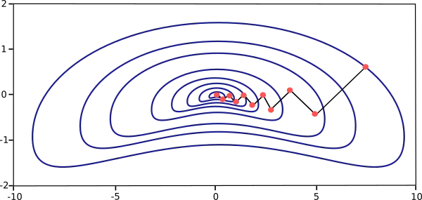
Full-batch gradient descent is useful as a baseline and for modest deterministic problems. Large deep networks generally use its mini-batch descendants rather than plain gradient descent.
Newton’s method
Newton’s method uses both the gradient and Hessian to account for local curvature. Instead of explicitly calculating an inverse, a numerical implementation solves
Near a well-behaved minimum, Newton’s method can converge in far fewer iterations than gradient descent. However, a network with \(D\) parameters has a \(D\times D\) Hessian. Storing it requires \(O(D^2)\) memory, and a dense factorization typically requires \(O(D^3)\) work.
The Hessian can also be indefinite away from a minimum, producing a direction that does not reduce the loss. Damping, trust regions, or a fallback descent direction are therefore needed in robust implementations.
Exact Newton training is mainly a conceptual reference or a specialist option for very small networks. Quasi-Newton and Gauss-Newton methods retain some curvature information at a lower cost.
Quasi-Newton methods: BFGS and L-BFGS
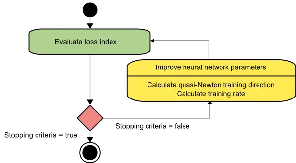
Quasi-Newton methods estimate curvature from successive parameter and gradient differences. They avoid evaluating the exact Hessian while constructing a search direction of the form
where \(\mathbf{G}^{(i)}\) approximates the inverse Hessian. A line search, commonly using an Armijo or Wolfe condition, chooses a step that provides sufficient decrease.
BFGS
The Broyden-Fletcher-Goldfarb-Shanno method updates a dense inverse-Hessian approximation using the latest parameter difference \(\Delta\boldsymbol{\theta}\) and gradient difference \(\Delta\mathbf{g}\). It often converges much faster than gradient descent on smooth, deterministic problems, but storing \(\mathbf{G}\) requires \(O(D^2)\) memory.
L-BFGS
Limited-memory BFGS is the same quasi-Newton family with a different storage strategy. It retains only the most recent \(m\) parameter and gradient difference pairs and reconstructs their action on the gradient when needed. This reduces optimizer-state memory to approximately \(O(mD)\), with \(m\) usually much smaller than \(D\).
BFGS is suitable for small-to-medium full-batch networks. L-BFGS extends the approach to larger deterministic parameter vectors, although both methods become less reliable when curvature pairs are estimated from unrelated noisy mini-batches.
Levenberg-Marquardt algorithm
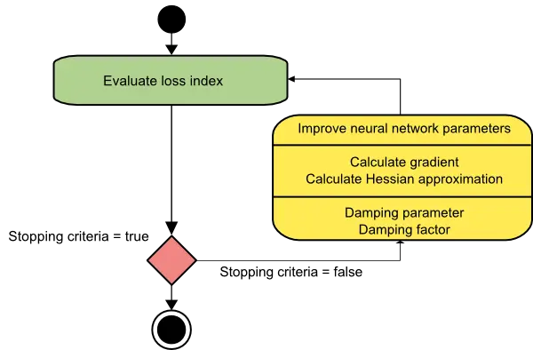
Levenberg-Marquardt is a specialized full-batch optimizer for smooth residual least-squares problems. Suppose a network produces residuals \(\mathbf{h}\) with one component per sample and output, and define
where \(B\) is the number of training samples and \(M\) is the number of outputs. If \(\mathbf{J}\) is the residual Jacobian, with shape \((BM)\times D\), the damped Gauss-Newton step solves
For small damping \(\lambda\), the update approaches Gauss-Newton. For large \(\lambda\), it approaches a small gradient-descent step. Successful candidate steps reduce the damping; rejected steps increase it.
Levenberg-Marquardt can converge rapidly for small, smooth regression networks. Its limitation is scale: explicitly storing \(\mathbf{J}\) and the \(D\times D\) Gauss-Newton matrix consumes substantial memory, and the dense linear solve is expensive.
The method applies directly to residual least-squares objectives, not to cross-entropy. When applied to the same residuals without changing other objective terms, MSE, SSE, and RMSE have the same minimizer; however, the LM calculation is formulated through the underlying residual vector rather than through an arbitrary scalar loss transformation.
Stochastic gradient descent
In contemporary deep learning, stochastic gradient descent usually means mini-batch SGD. At each iteration, it calculates a gradient \(\mathbf{g}_{B}^{(i)}\) from a batch of \(B\) samples:
A mini-batch gradient is noisy, but it is much cheaper than a full-dataset gradient and can be evaluated efficiently using parallel hardware. Batch size and learning rate must be chosen together.
Momentum
Momentum accumulates a velocity vector that smooths oscillations and reinforces directions that remain consistent across batches:
A momentum coefficient of \(\mu=0.9\) is a common starting point, not a universal optimum. Momentum adds one state value per parameter.
Nesterov momentum
Nesterov momentum evaluates the gradient with respect to a look-ahead position, allowing the optimizer to correct its direction before completing the momentum step. Modern libraries often use an algebraically rearranged implementation that avoids a second gradient calculation.
Learning-rate schedules
SGD performance depends strongly on its learning-rate schedule. Step decay, exponential decay, cosine decay, and warm-up followed by decay are common choices. Line searches are rarely used because batch-to-batch noise makes them unreliable.
SGD with momentum remains attractive for large networks when optimizer-state memory is constrained or when a carefully tuned SGD recipe provides strong validation performance. It generally needs more learning-rate tuning than Adam.
Adam and AdamW
Adam adapts the step for every parameter using exponential moving averages of the gradient and squared gradient. At iteration \(i\),
Because both averages start at zero, Adam applies bias correction:
The parameter update is
where all divisions and square roots are element-wise. The original defaults \(\beta_1=0.9\), \(\beta_2=0.999\), \(\epsilon=10^{-8}\), and \(\eta=10^{-3}\) are useful starting values, but the learning rate and schedule still require validation.
Adam is a robust mini-batch baseline for large, non-convex problems and can work well with noisy or sparse gradients. Its two moment estimates require two optimizer-state values per parameter, twice the state of momentum SGD.
AdamW and decoupled weight decay
For ordinary SGD, adding an L2 penalty to the loss is closely related to multiplying the parameters by a weight-decay factor. This equivalence does not hold for Adam because its adaptive denominator rescales the L2 contribution differently for every parameter.
AdamW decouples weight decay from the adaptive gradient calculation:
This separation makes the learning rate and weight-decay coefficient easier to reason about independently. AdamW is a common choice for transformers and other modern deep networks when explicit weight decay is desired.
Optimizer comparison
The following table compares optimizer-state memory rather than total training memory. Parameters, gradients, activations, temporary tensors, and dataset storage are additional costs. Here, \(D\) is the number of trainable parameters, \(m\) is the L-BFGS history length, and \(BM\) is the number of residuals in a full LM batch.
| Optimizer family | Typical batch regime | Information used | Extra optimizer state | Best suited for | Main limitation |
|---|---|---|---|---|---|
| Gradient descent | Full batch | Gradient | Minimal | Baselines and modest deterministic problems | Slow on poorly conditioned losses |
| Newton | Full batch | Gradient and exact Hessian | \(D^2\) | Very small smooth problems | Hessian storage and dense solve |
| Quasi-Newton BFGS / L-BFGS | Full batch | Gradient and curvature pairs | \(D^2\) / approximately \(2mD\) | Small-to-medium smooth deterministic problems | Curvature estimates degrade with noisy batches |
| Levenberg-Marquardt | Full batch | Residual Jacobian | \(BMD+D^2\) | Small residual least-squares networks | Specialized loss and high memory use |
| SGD with momentum | Mini-batch | Batch gradient and velocity | \(D\) | Large networks; memory-conscious training | Sensitive to learning rate and schedule |
| Adam / AdamW | Mini-batch | First and second gradient moments | \(2D\) | General deep-learning baseline; transformers | More optimizer state and regularization choices |
There is no universal ranking by “speed.” Time per update, number of updates, hardware utilization, final validation performance, and hyperparameter budget can all change the result. Comparisons should report wall-clock time to a common validation target, peak memory, final test performance, and variability across repeated runs.
Product note: Neural Designer documents gradient descent, Newton, quasi-Newton, Levenberg-Marquardt, SGD, and Adam in its training strategy guide. Availability of individual variants such as L-BFGS or AdamW can depend on the installed product version.
How to choose an optimizer
- Start with the loss and scale. If the objective is smooth residual least squares and both the network and dataset are modest, Levenberg-Marquardt is a strong candidate.
- For a smooth general full-batch problem, try quasi-Newton. Use BFGS when its dense state fits comfortably in memory and L-BFGS when the full approximation is too large.
- For large datasets or deep networks, use mini-batches. Adam is a reliable starting point; use AdamW when decoupled weight decay is available and appropriate.
- Use SGD with momentum when memory matters or when the workload has a proven SGD recipe. Expect to tune the learning rate, momentum, batch size, and schedule together.
- Reserve exact Newton for very small or specialist problems. It is valuable for understanding curvature, but its dense Hessian rarely scales to contemporary networks.
Optimizer choice is only one part of training. Initialization, feature scaling, normalization, batch size, mixed precision, gradient clipping, regularization, learning-rate scheduling, and validation-based early stopping can matter as much as the optimizer name.
A practical comparison keeps the model, data split, loss, stopping budget, and evaluation metric fixed, then tunes each optimizer fairly and compares validation performance, elapsed time, and peak memory.
Emerging optimizers
AdamW and momentum SGD remain strong reference methods, but optimizer research continues to address memory and curvature at scale:
- Adafactor factors the second-moment accumulator for matrix parameters, reducing optimizer-state memory in large transformer models.
- Shampoo uses tensor-structured preconditioners to capture more geometry than diagonal adaptive methods.
- Lion uses sign-based momentum updates and stores one momentum state instead of Adam’s two moments.
- Sophia applies a clipped update preconditioned by a lightweight diagonal Hessian estimate for language-model pretraining.
- Muon orthogonalizes updates for matrix-valued hidden-layer parameters and is being studied as an alternative for large language-model training.
These methods are promising but task-specific. They should be presented as research and engineering options, not as universal replacements for AdamW, SGD, quasi-Newton, or Levenberg-Marquardt.
Conclusions
Modern neural-network optimization spans two complementary regimes. Full-batch curvature-aware methods can converge rapidly when the model and dataset are modest. Mini-batch methods trade exact gradient information for scalable, hardware-efficient updates.
- Use Levenberg-Marquardt for small residual least-squares networks.
- Use BFGS or L-BFGS for smooth deterministic problems that benefit from curvature information.
- Use Adam or AdamW as practical starting points for large deep networks.
- Use SGD with momentum when its memory efficiency or task-specific generalization makes it preferable.
The best choice is the optimizer that reaches the required validation quality within the available time and memory budget. That choice should be established by a fair experiment rather than by a universal ranking.
References
- Sutskever, I. et al. (2013). On the importance of initialization and momentum in deep learning.
- Nocedal, J. (1980). Updating quasi-Newton matrices with limited storage.
- Marquardt, D. W. (1963). An algorithm for least-squares estimation of nonlinear parameters.
- Kingma, D. P. and Ba, J. (2015). Adam: A method for stochastic optimization.
- Loshchilov, I. and Hutter, F. (2019). Decoupled weight decay regularization.
- Shazeer, N. and Stern, M. (2018). Adafactor: Adaptive learning rates with sublinear memory cost.
- Gupta, V. et al. (2018). Shampoo: Preconditioned stochastic tensor optimization.
- Chen, X. et al. (2023). Symbolic discovery of optimization algorithms.
- Liu, H. et al. (2023). Sophia: A scalable stochastic second-order optimizer for language model pre-training.
- Liu, J. et al. (2025). Muon is scalable for LLM training.