Learning

Build a neural network in 7 steps

In this tutorial, you will build a neural network that learns a simple nonlinear relationship from a small CSV file. The example contains one input, x, and one target, y, related by y = x².

Download example dataset

To complete this example, follow these steps:

Create approximation model
Configure data set
Set network architecture
Train neural network
Improve generalization performance
Test results
Deploy model

Create approximation model

Open Neural Designer. The start page is shown.

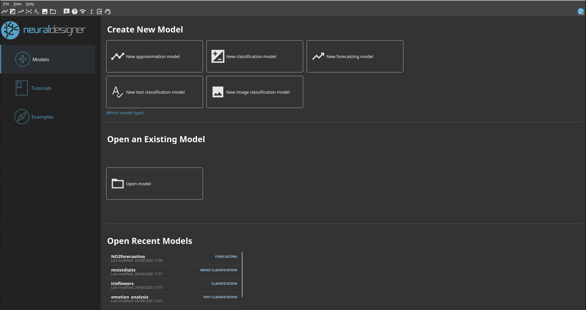
Click New approximation model. Then save the project file in the same folder as the data file. Neural Designer now displays the main workspace.

Configure data set

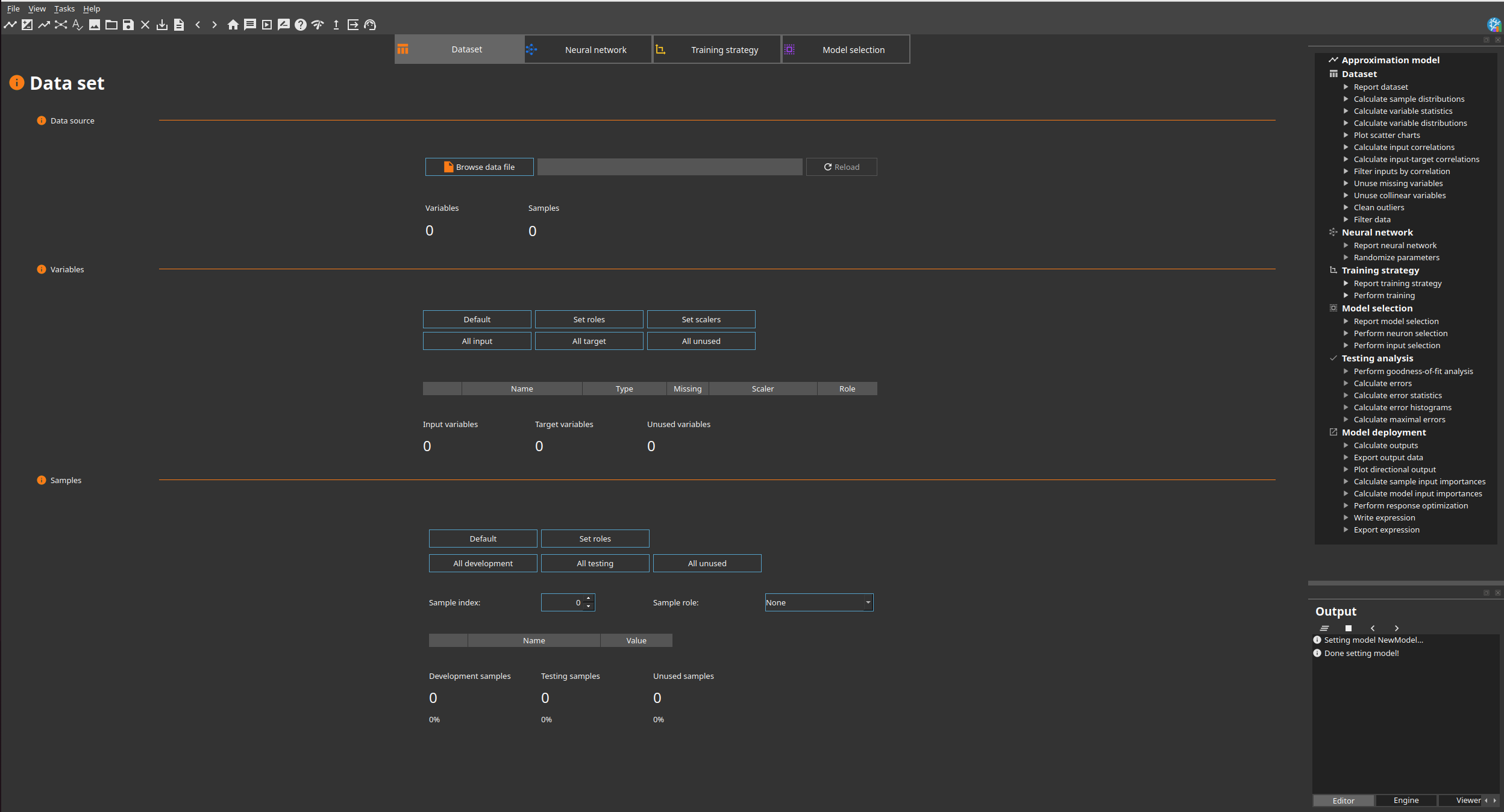
After creating the model, go to the Data set page and click Browse data file. For this tutorial, a simple CSV file has been opened as an example.

Download example dataset

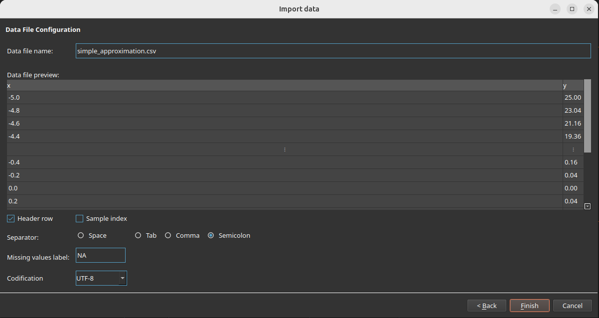
The Import data window previews the contents and the detected settings. In this example, the file has a header row, uses a semicolon separator, has no sample index and uses UTF-8 encoding. After checking the preview, click Finish.

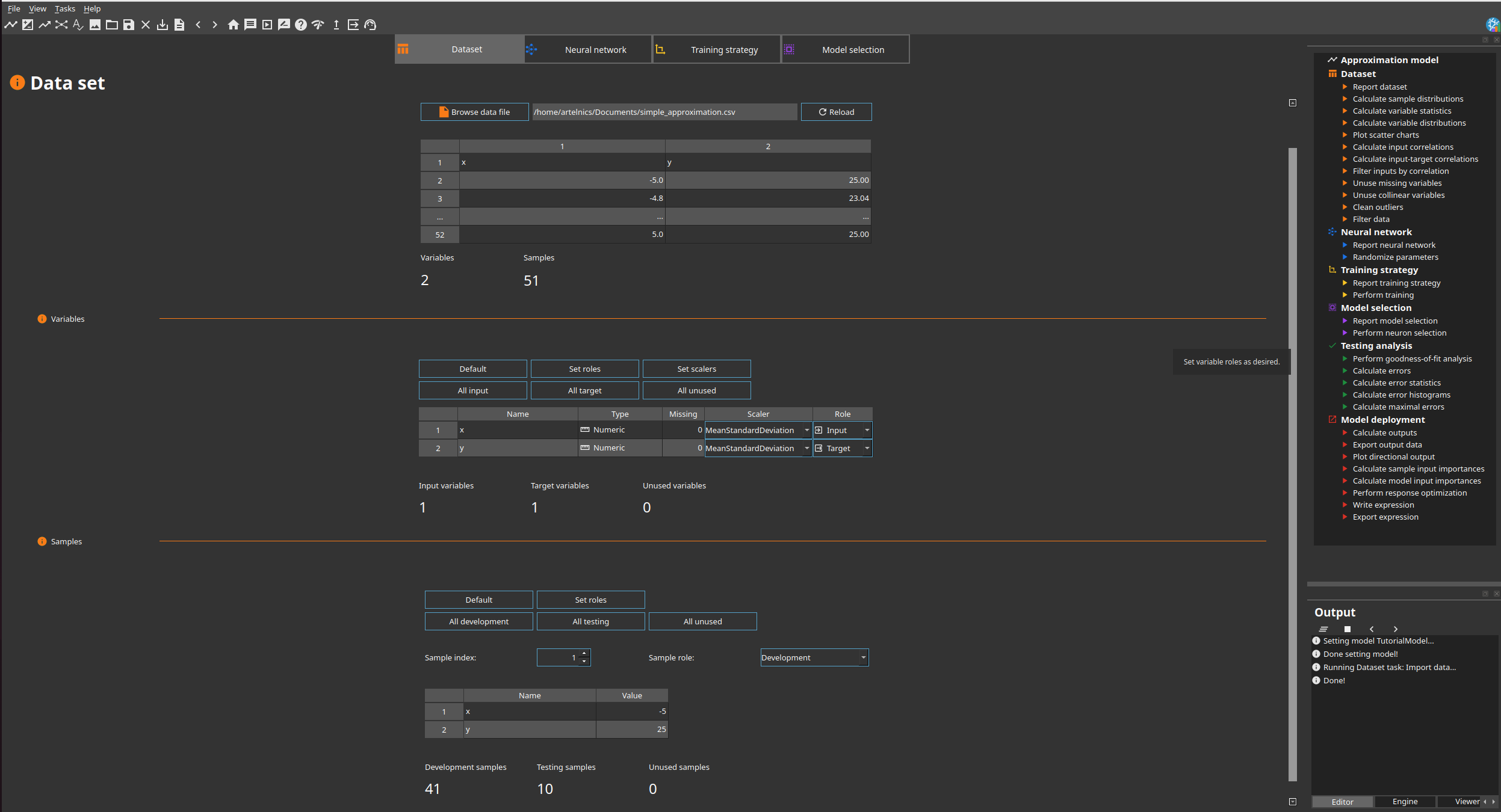
The data set contains 51 samples and two numeric variables, with no missing values:

x is the input variable.
y is the target variable.

Neural Designer applies the MeanStandardDeviation scaler to both variables. The default sample split assigns 41 samples to development and 10 to testing; no samples are unused.

Select a sample index to inspect its values and role in the lower table.

After configuring the data set, open Task Manager > Data set > Plot scatter charts. The Viewer plots the target y against the input x.

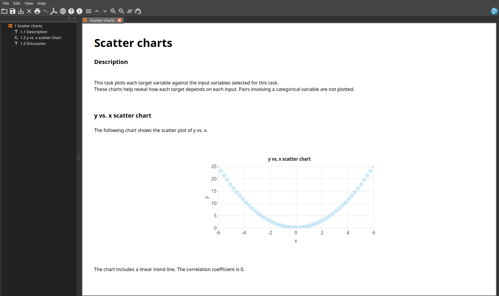
The parabolic shape represents y = x². Its linear correlation coefficient is 0 because the relationship is symmetric and nonlinear, illustrating why linear correlation alone cannot reveal every dependency.

You can also evaluate data quality by running additional dataset analysis tasks.

Set network architecture

Next, click on the Neural network tab to configure the approximation model. The page displays its current layers and architecture.

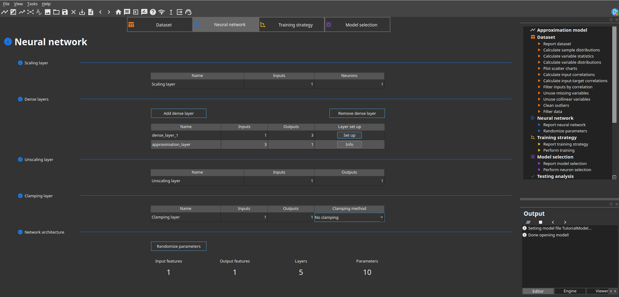
The example uses one input feature (x) and one target (y). Neural Designer creates five layers by default:

One scaling layer with 1 input and 1 neuron.
Two dense layers: a hidden layer with 3 neurons and an output layer with 1 neuron.
One unscaling layer with 1 input and 1 output.
One clamping layer with 1 input and 1 output. Its default method is No clamping.

The hidden dense layer uses a hyperbolic tangent activation function. The output dense layer uses a linear activation function. The summary reports 1 input feature, 1 output feature, 5 layers and 10 parameters. Keep these default settings.

To visualize the network architecture, run Neural network > Report neural network from the task tree. The Viewer window displays the complete architecture.

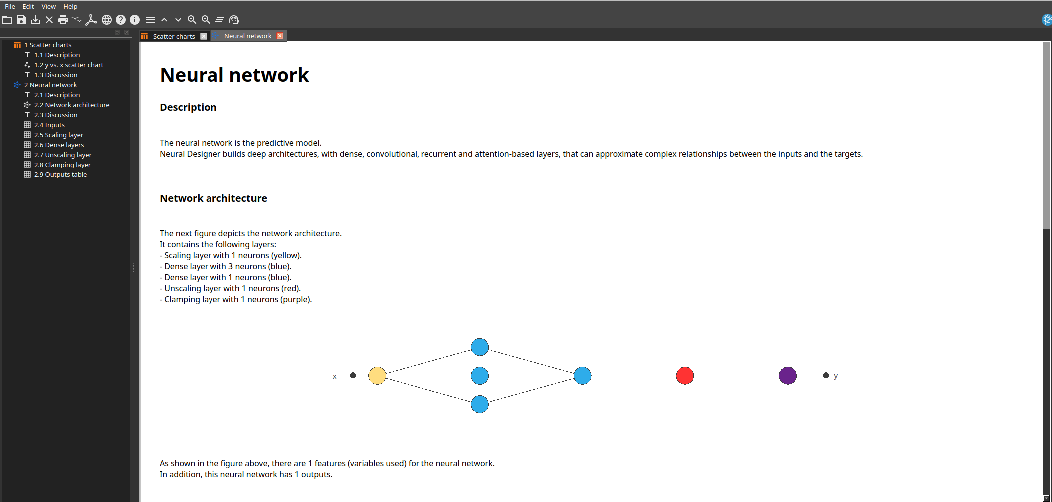
The report shows x entering the scaling layer (yellow), followed by the two dense layers (blue), the unscaling layer (red), and the clamping layer (purple), which produces y.

Train neural network

Open the Training strategy tab. This page configures the loss index and the optimization algorithm.

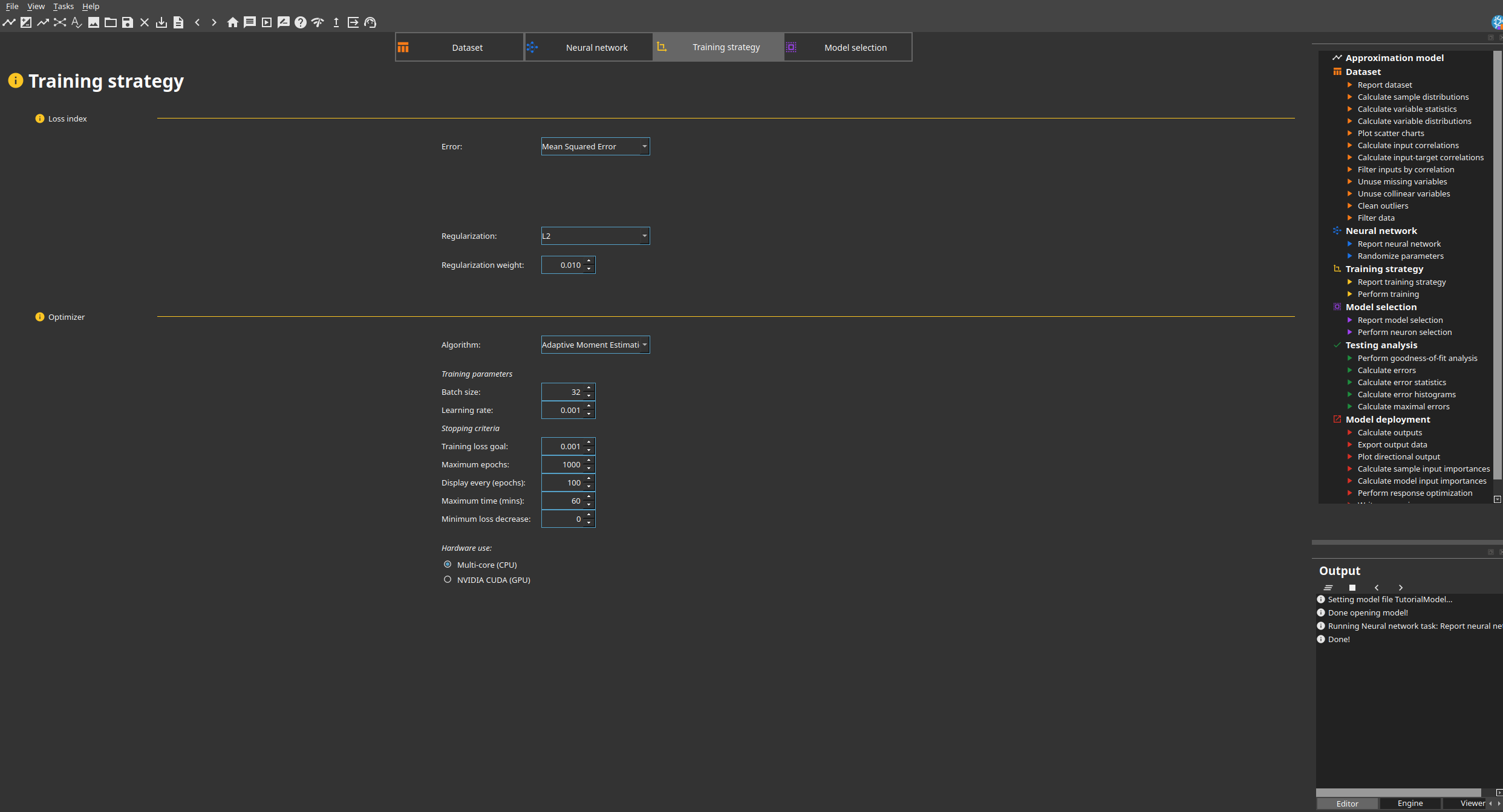
For this example, keep the displayed settings:

Mean squared error as the error method.
L2 regularization with a weight of 0.010.
Adaptive moment estimation (Adam) with a batch size of 32 and a learning rate of 0.001.
A maximum of 1000 epochs using the multi-core CPU.

Run Training strategy > Perform training from the task tree. The optimizer minimizes the loss index and adjusts the network parameters to fit y = x².

For a practical comparison of gradient descent, quasi-Newton, Levenberg-Marquardt, SGD, Adam and AdamW, see our neural network optimizer guide.

Improve generalization performance

Open the Model selection tab to configure neuron and input selection.

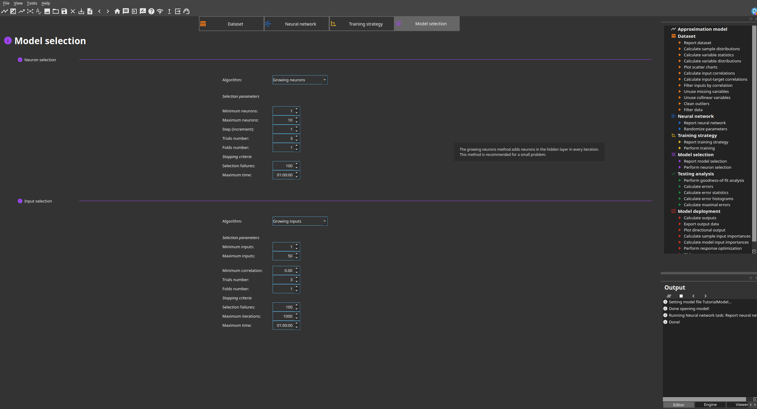
For this example, keep Growing neurons with a minimum of 1 neuron, a maximum of 10, a step of 1 and 3 trials. Input selection is not needed because x is the only input.

Run Model selection > Perform neuron selection from the task tree. The Viewer displays the growing-neurons report.

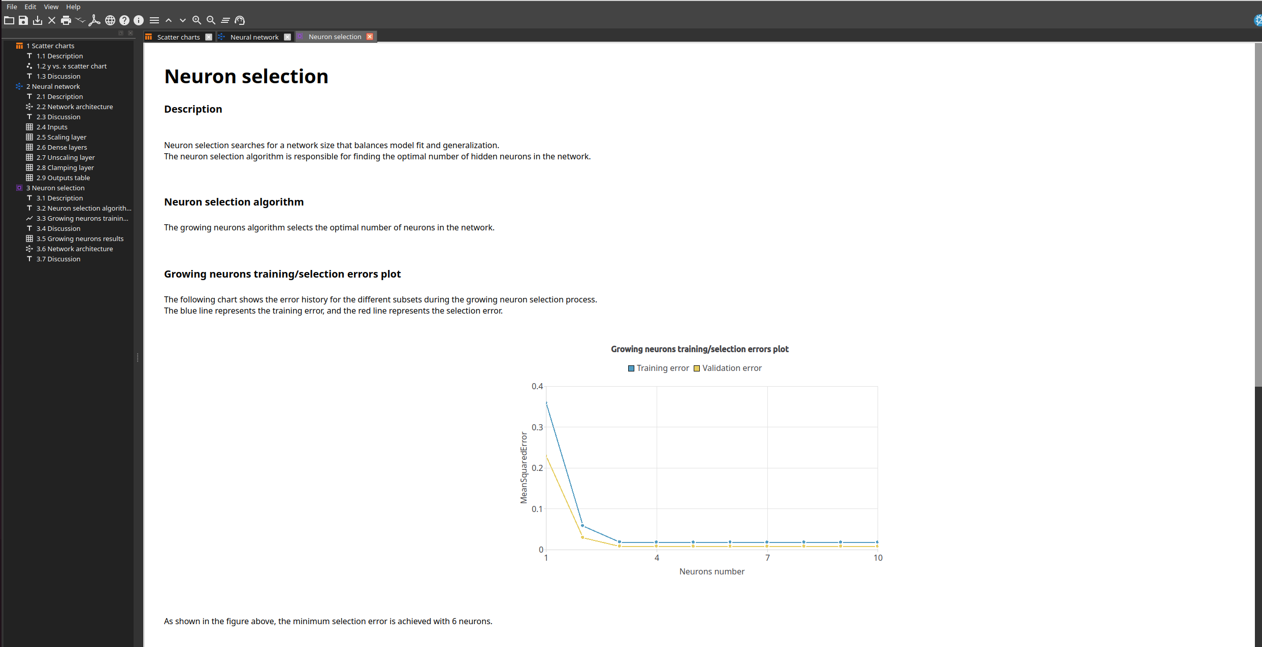
The training and selection errors decrease rapidly. The minimum selection error is achieved with 6 neurons.

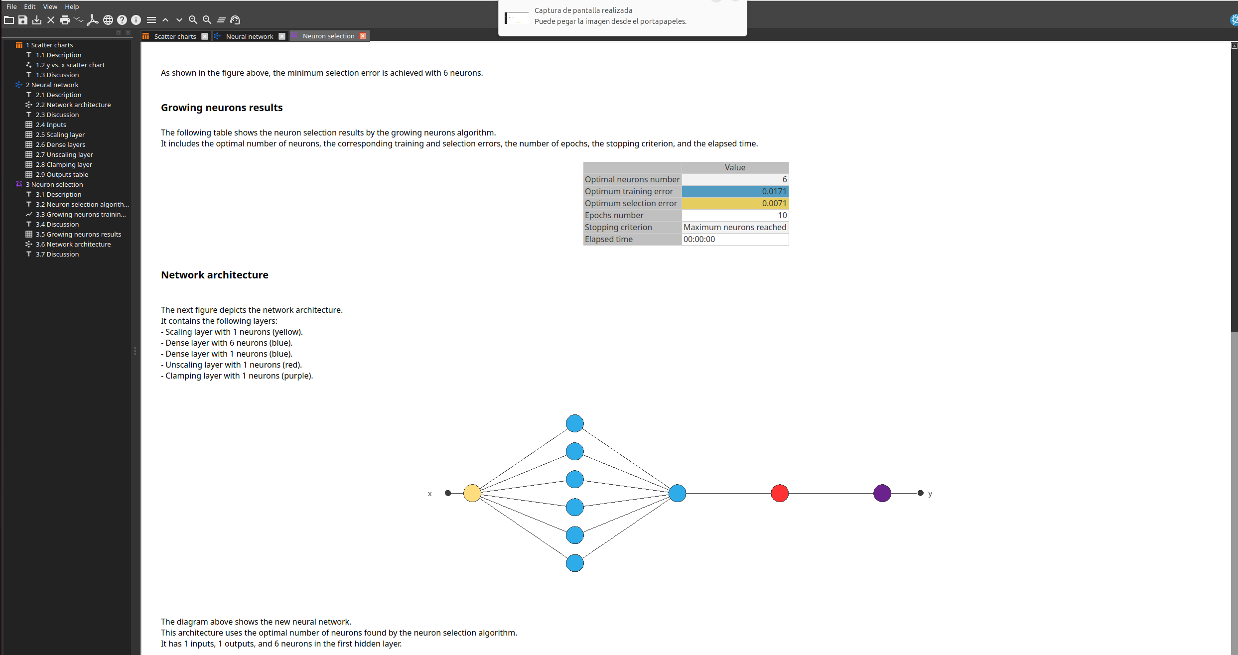
The results report shows 6 optimal neurons, a training error of 0.0171, a selection error of 0.0071 and 10 epochs. Neural Designer updates the network architecture to one hidden layer with 6 neurons and one output neuron. The resulting neural network is already trained.

Test results

Open Testing analysis to evaluate the trained model on the testing samples, which were not used to fit its parameters.

Run Testing analysis > Perform goodness-of-fit analysis from the task tree. The Viewer displays the coefficient of determination and the predicted-versus-actual chart.

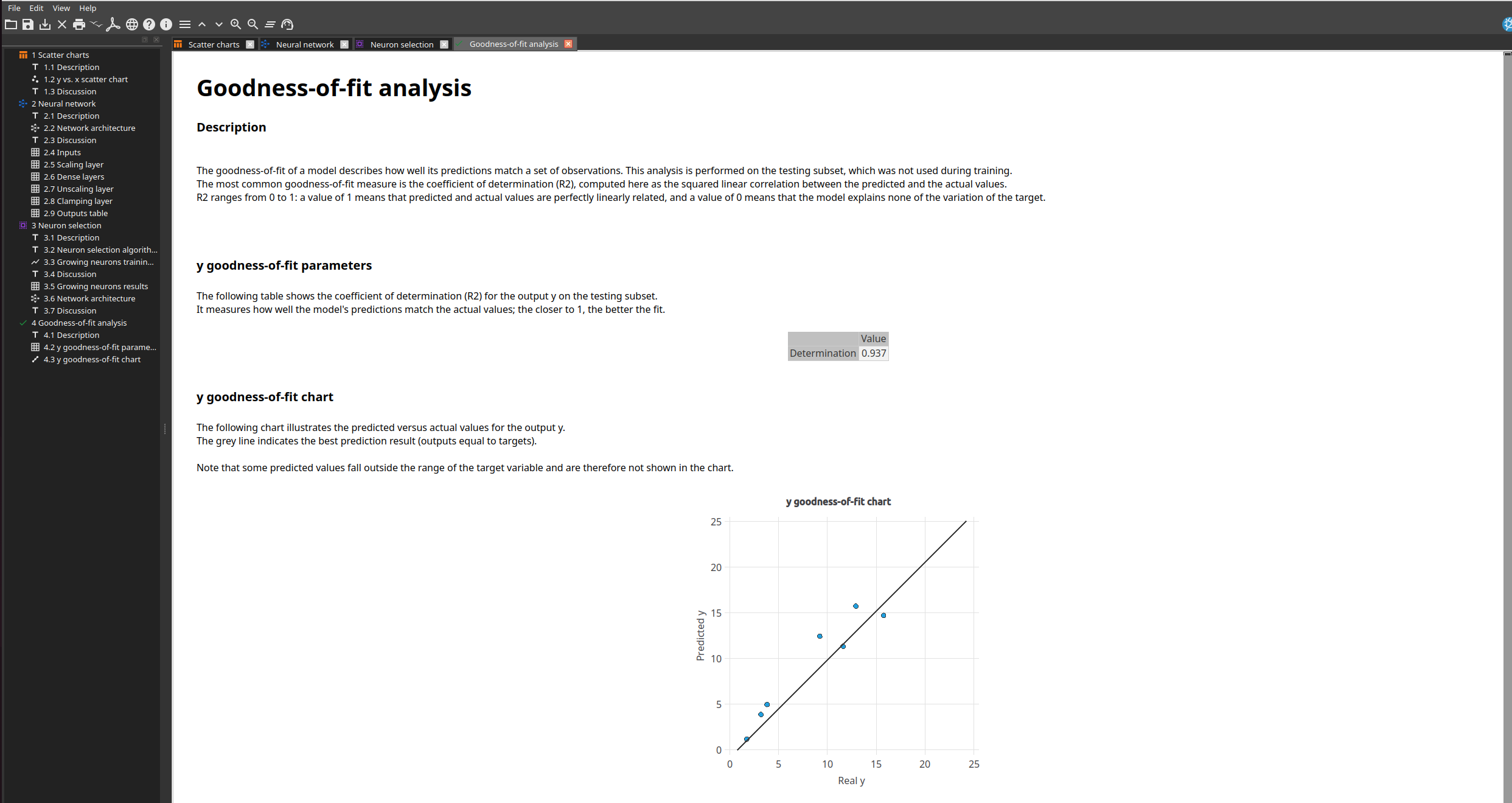
The goodness-of-fit analysis reports R² = 0.937 for y. The blue points compare predicted and actual values, while the grey line represents perfect predictions. Points closer to that line indicate a better fit.

Deploy model

Once the model has been tested, open Model deployment to generate predictions, analyze its responses and export the model.

Run Model deployment > Plot directional output from the task tree. This task varies one input while keeping the others fixed at a reference point.

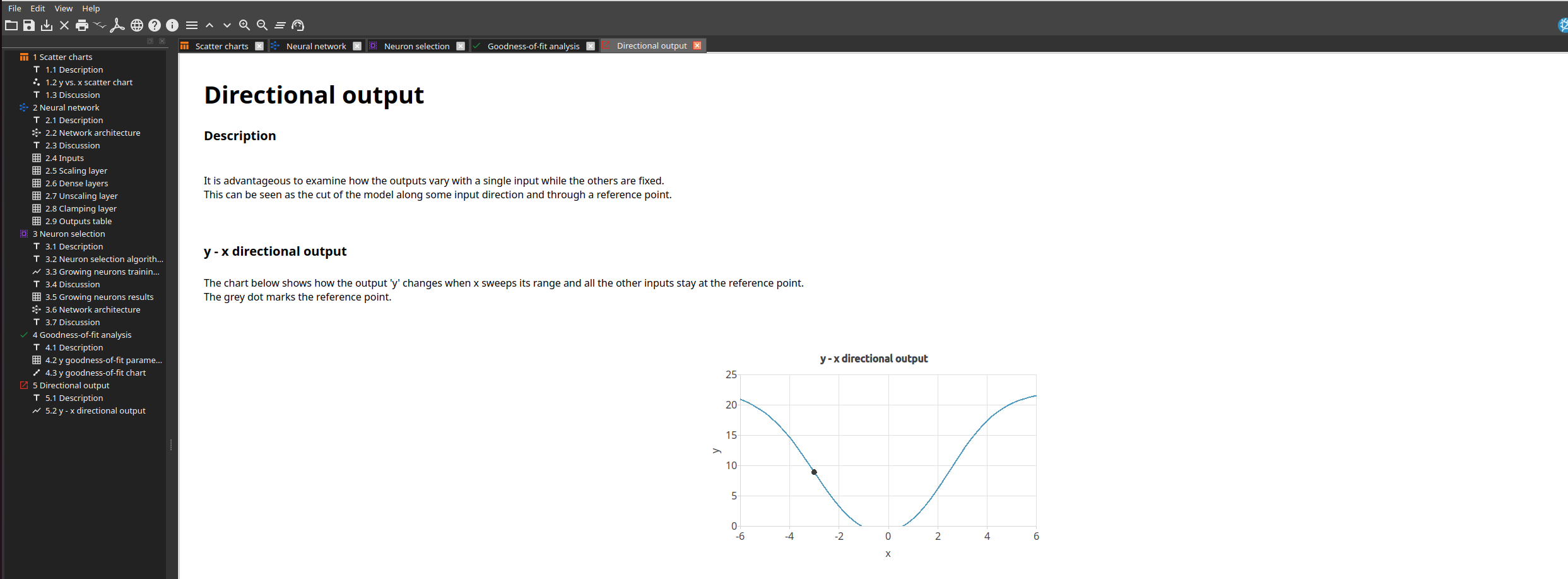
Because this example has only one input, the chart directly shows the response y(x) learned by the network. The grey point marks the reference input.

Run Model deployment > Export expression to save the complete model as Python code. Instantiate NeuralNetwork and call calculate_outputs([...]) for one prediction or calculate_batch_output(...) for a NumPy batch.

'''
Artificial Intelligence Techniques SL
artelnics@artelnics.com

Model exported to Python. Use NeuralNetwork().calculate_outputs([...]).

Input Names:
	0) x

For batch prediction (input must be np.ndarray):
	nn.calculate_batch_output(np.array([[1], [4]]))
'''
import math
import numpy as np
import pandas as pd

class NeuralNetwork:

	def __init__(self):
		self.inputs_number = 1
		self.input_names = ['x']

	@staticmethod
	def Identity(x):
		return x

	@staticmethod
	def Tanh(x):
		return np.tanh(x)

	def calculate_outputs(self, inputs):
		x = inputs[0]

		scaled_x = x*0.3396831453+1.905571523e-08
		dense_layer_1_output_0 = self.Tanh( 1.151840448 + (-1.392787814*scaled_x) )
		dense_layer_1_output_1 = self.Tanh( -1.355468988 + (-1.329861999*scaled_x) )
		dense_layer_1_output_2 = self.Tanh( -0.6183619499 + (0.009102747776*scaled_x) )
		dense_layer_1_output_3 = self.Tanh( -0.3707145751 + (0.01256038155*scaled_x) )
		dense_layer_1_output_4 = self.Tanh( -0.02022263408 + (-0.03428416327*scaled_x) )
		dense_layer_1_output_5 = self.Tanh( -0.001989847049 + (0.05457909405*scaled_x) )
		approximation_layer_output_0 = self.Identity( 1.264135718 + (-1.791464567*dense_layer_1_output_0) + (1.778391838*dense_layer_1_output_1) + (-0.6996221542*dense_layer_1_output_2) + (-0.3780626953*dense_layer_1_output_3) + (-0.04951105267*dense_layer_1_output_4) + (-0.07944823802*dense_layer_1_output_5) )
		unscaling_layer_output_0 = approximation_layer_output_0*7.747230053+8.666669846
		y = unscaling_layer_output_0
		outputs = [y]
		return outputs

	def calculate_batch_output(self, input_batch):
		output_batch = np.zeros((len(input_batch), 1))
		for i in range(len(input_batch)):
			inputs = list(input_batch[i])
			output = self.calculate_outputs(inputs)
			output_batch[i] = output
		return output_batch

def main():

	# Introduce your input values here
	x = 0  # x

	# --- Data conversion (DO NOT modify) ---
	inputs = []
	inputs.append(x)

	nn = NeuralNetwork()
	outputs = nn.calculate_outputs(inputs)
	print(outputs)

if __name__ == "__main__":
	main()

To learn more, see the next example:

Classification of iris flowers from sepal and petal dimensions.