Classification of iris flowers is perhaps the best-known example of machine learning. The aim is to classify iris flowers among three species (Setosa, Versicolor, or Virginica) from the sepals’ and petals’ length and width measurements. Here, we design a model that makes proper classifications for new flowers. In other words, one which exhibits good generalization.
Contents
- Application type.
- Data set.
- Neural network.
- Training strategy.
- Model selection.
- Testing analysis.
- Model deployment.
- Tutorial video.
The iris data set contains fifty instances of each of the three species.
This example is solved with the data science and machine learning platform Neural Designer. Use the free trial to follow it step by step.
1. Application type
This is a classification project. Indeed, the variable to be predicted is categorical (setosa, versicolor, or virginica).
The goal is to model class membership probabilities conditioned on the flower features.
2. Data set
The first step is to prepare the data set. This is the source of information for the classification problem. For that, we need to configure the following concepts:
- Data source.
- Variables.
- Instances.
The data source is the file iris_flowers.csv. It contains the data for this example in comma-separated values (CSV) format. The number of columns is 5, and the number of rows is 150.
The variables are:
- sepal_length: Sepal length, in centimeters, used as input.
- sepal_width: Sepal width, in centimeters, used as input.
- petal_length: Petal length, in centimeters, used as input.
- petal_width: Petal width, in centimeters, used as input.
- class: Iris Setosa, Versicolor, or Virginica, used as the target.
Note that neural networks work with numbers. In this regard, the categorical variable “class” is transformed into three numerical variables as follows:
- iris_setosa: 1 0 0.
- iris_versicolor: 0 1 0.
- iris_virginica: 0 0 1.
The instances are divided into training, selection, and testing subsets. They represent 60% (90), 20% (30), and 20% (30) of the original instances, respectively, and are randomly split.
We can calculate the distributions of all variables. The following figure is the pie chart for the iris flower class.
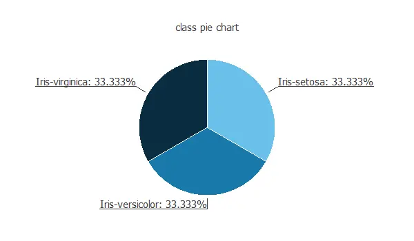
As we can see, the target is well-distributed. Indeed, there is the same number of Virginica, Setosa, and Versicolor samples.
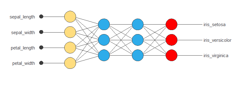
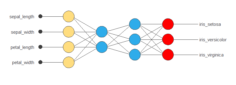
3. Neural network
The second step is to choose a neural network. For classification problems, it is usually composed by:
- A scaling layer.
- Two perceptron layers.
- A probabilistic layer.
The neural network must have four inputs since the data set has four input variables (sepal length, sepal width, petal length, and petal width).
The scaling layer normalizes the input values. All input variables have normal distributions, so we use the mean and standard deviation scaling method.
Here, we use 2 perceptron layers:
- The first layer has 4 inputs, 3 neurons, and a logistic activation function.
- The second layer has 3 inputs, 3 neurons, and a logistic activation function.
The probabilistic layer allows us to interpret the outputs as probabilities. In this regard, all outputs are between 0 and 1, and their sum is 1. The softmax probabilistic method is used here.
The neural network has three outputs since the target variable contains three classes (Setosa, Versicolor, and Virginica).
The next figure is a graphical representation of this classification neural network:
4. Training strategy
The fourth step is to set the training strategy, which is composed of:
- Loss index.
- Optimization algorithm.
The loss index chosen for this application is the normalized squared error with L2 regularization.
The error term fits the neural network to the training instances of the data set. The regularization term makes the model more stable and improves generalization.
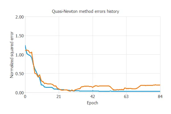
The optimization algorithm searches for the neural network parameters that minimize the loss index. The quasi-Newton method is chosen here.
The following chart shows how the training and selection errors decrease with the epochs during training.
The final values are training error = 0.005 NSE (blue) and selection error = 0.195 NSE (orange).
5. Model selection
The objective of model selection is to find the network architecture with the best generalization properties. That is, that which minimizes the error on the selected instances of the data set.
We want to find a neural network with a selection error of less than 0.195 NSE, the value we have achieved so far.
Order selection algorithms train several network architectures with a different number of neurons and select that with the most minor selection error.
The incremental order method starts with a few neurons and increases the complexity at each iteration. The following chart shows the training error (blue) and the selection error (orange) as a function of the number of neurons.
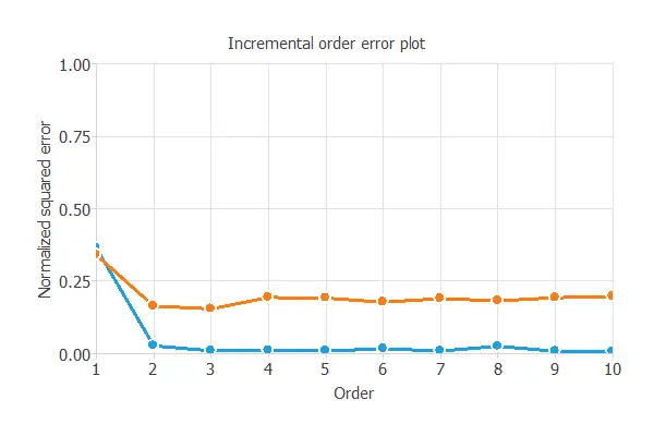
We can see that the order yielding the minimum selection error is two. Therefore, we select the neural network with two neurons in the first perceptron layer.
6. Testing analysis
The purpose of the testing analysis is to validate the generalization performance of the model. Here, we compare the neural network outputs to the corresponding targets in the testing instances of the data set.
In the confusion matrix, the rows represent the targets (or real values) and the columns the corresponding outputs (or predictive values). The diagonal cells show the correctly classified samples. The off-diagonal cells show the misclassified samples.
| Predicted setosa | Predicted versicolor | Predicted virginica | |
|---|---|---|---|
| Real setosa | 10 (33.3%) | 0 | 0 |
| Real versicolor | 0 | 11 (36.7%) | 0 |
| Real virginica | 0 | 1 (3.33%) | 8 (26.7%) |
Here we can see that all testing instances are well classified, but one. In particular, the neural network has classified one flower as Virginica being Versicolor. Note that the confusion matrix depends on the particular testing instances we have.
The confusion matrix allows us to calculate the model’s accuracy and error:
- Classification accuracy: 96.67%.
- Error rate: 3.33%.
7. Model deployment
The neural network is now ready to predict outputs for inputs it has never seen. This process is called model deployment.
To classify a given iris flower, we calculate the neural network outputs from the lengths and withs of its sepals and petals. For instance:
For this particular case, the neural network would classify that flower as being of the versicolor species since it has the highest probability.
The mathematical expression of the trained neural network is listed below.
scaled_sepal_length = 2*(sepal_length-4.3)/(7.9-4.3)-1;
scaled_sepal_width = 2*(sepal_width-2)/(4.4-2)-1;
scaled_petal_length = 2*(petal_length-1)/(6.9-1)-1;
scaled_petal_width = 2*(petal_width-0.1)/(2.5-0.1)-1;

y_1_1 = logistic(-8.9598 + (scaled_sepal_length*1.58675) + (scaled_sepal_width*-4.05111)
+ (scaled_petal_length*10.7863) + (scaled_petal_width*12.7033));

y_1_2 = logistic(1.8634 + (scaled_sepal_length*-0.789934) + (scaled_sepal_width*-2.53173)
+ (scaled_petal_length*3.47617) + (scaled_petal_width*5.04384));

non_probabilistic_iris_setosa = logistic(3.43875+ (y_1_1*0.950696)+ (y_1_2*-8.35938));
non_probabilistic_iris_versicolor = logistic(-4.41592+ (y_1_1*-11.319)+ (y_1_2*9.58436));
non_probabilistic_iris_virginica = logistic(-7.10419+ (y_1_1*11.5014)+ (y_1_2*1.88165));

(iris_setosa,iris_versicolor,iris_virginica) = softmax(non_probabilistic_iris_setosa,
                                                       non_probabilistic_iris_versicolor,
                                                       non_probabilistic_iris_virginica);
We can implement this expression in any programming language to obtain the output for our input.
8. Video tutorial
Watch the step-by-step video tutorial of this example solved with Neural Designer.