Screen satellite-image segments for tree-wilt signatures
This reproducible classification study uses five QuickBird spectral and texture descriptors to distinguish wilt-labelled segments from other land cover. After an explicit 3-IQR outlier-cleaning step, the selected 5–4–1 network classifies 85 of 113 held-out rows correctly (75.2%; ROC AUC 0.819). The result is an internal benchmark for a deliberately rebalanced tutorial subset, not a validated forest-health monitoring system.
1. Scientific objective
The objective is to reproduce a binary remote-sensing classifier that assigns a wilt score to a segmented QuickBird image object. The source study targeted foliage discolouration associated with Japanese oak wilt and Japanese pine wilt. In a research workflow, the model can help prioritize image segments for map review and field inspection; it does not identify a pathogen or confirm disease in an individual tree.
Rank image objects from routinely derived spectral and panchromatic texture summaries.
Expose the exact subset construction, outlier rule, exclusions and random split before modelling.
Report sensitivity, specificity and false-negative counts rather than accuracy alone.
wilt; the page does not model disease progression, causal agents, infestation severity or individual-tree survival.2. Data and provenance
The downloadable tree_wilt.csv contains 574 rows, five numeric inputs and one binary target, with no missing values.
| CSV field | Model role | Definition | Unit or coding |
|---|---|---|---|
glcm | Input | Mean grey-level co-occurrence-matrix texture statistic from the panchromatic band | Image-derived statistic |
green | Input | Mean green-band value inside the image segment | Source-image digital value |
red | Input | Mean red-band value inside the image segment | Source-image digital value |
nir | Input | Mean near-infrared-band value inside the image segment | Source-image digital value |
pan_band | Input | Standard deviation of panchromatic-band values inside the segment | Source-image digital value |
wilt | Target | Supplied segment class | 1 = diseased-tree segment; 0 = other land cover |
Derived tutorial subset
The UCI release provides separate training and testing files. This tutorial table is a derived, rebalanced subset: it contains all 500 rows from the source testing file plus the 74 diseased-tree rows from the source training file. It excludes the 4,265 other-land-cover rows from that training file. The resulting table contains 261 positive and 313 negative rows and must not be compared directly with results from the original UCI split.
Outlier cleaning before modelling
Neural Designer applies Tukey’s rule to the numeric variables: values outside [Q1 − 3×IQR, Q3 + 3×IQR] are flagged. The per-variable counts are shown below; they overlap, so they do not sum to the number of excluded rows.
| Variable | Flagged values |
|---|---|
glcm | 0 |
green | 6 |
red | 4 |
nir | 1 |
pan_band | 1 |
wilt | 0 |
Seven overlapping rows (1.22% of the table) are marked unused. All seven have wilt = 0. The model therefore uses 567 rows: 261 positive and 306 negative.
Interactive chart: green distribution. Enable JavaScript to explore it.
Interactive chart: green distribution. Enable JavaScript to explore it.
| Project role | Rows | Wilt | Other land cover | Purpose |
|---|---|---|---|---|
| Training | 341 | 150 | 191 | Estimate model parameters |
| Selection | 113 | 62 | 51 | Compare hidden-layer sizes |
| Testing | 113 | 49 | 64 | Report final internal performance |
| Unused after cleaning | 7 | 0 | 7 | Excluded before fitting |
3. Model
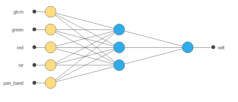
The initial network standardizes the five inputs, passes them through one dense layer with three tanh neurons and returns one sigmoid score. The 5–3–1 architecture contains 22 trainable parameters and is used as the starting point before hidden-layer selection.
4. Training strategy
The classifier minimizes class-weighted squared error with the quasi-Newton method. The stored configuration uses positive and negative weights of 1.0862 and 0.9265, respectively, and no explicit regularization.
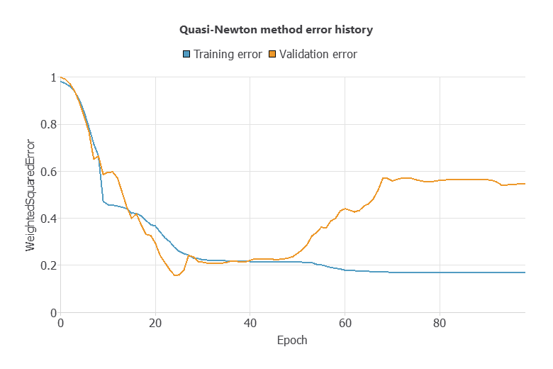
For the initial three-neuron network, training error falls from 0.982 to 0.169 over 98 epochs. Selection error reaches its lowest region much earlier—approximately 0.158 near epoch 24—and then rises to 0.548. This divergence is evidence of overfitting in the displayed run; it is one reason not to judge the model from training loss alone.
5. Model selection and baseline
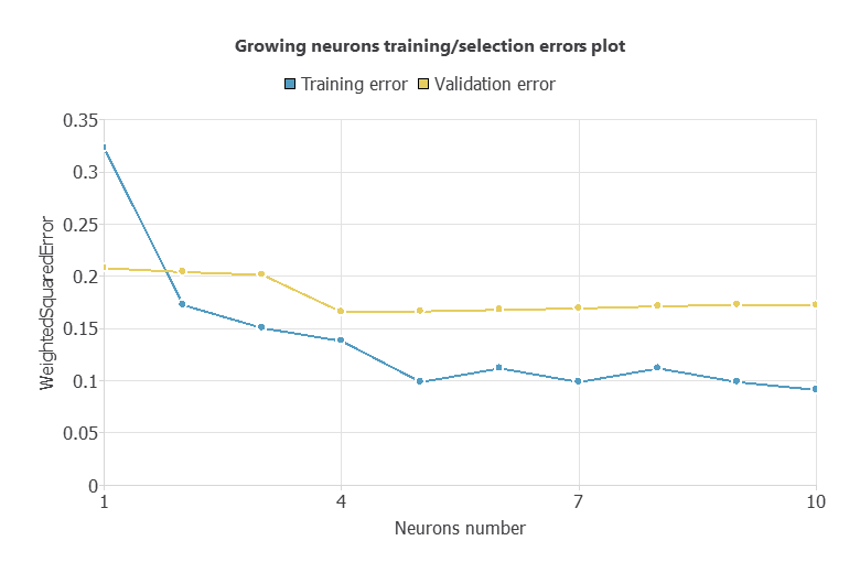
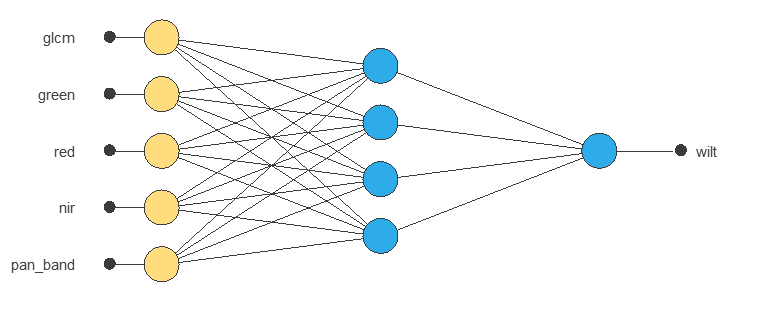
Growing-neurons selection evaluates hidden-layer sizes from one to ten, with three trials per size. The lowest reported selection error is 0.1657 at four hidden neurons; the corresponding training error is 0.1380.
Selected architecture
The selected 5–4–1 network has 29 trainable parameters and is the model used for the final testing analysis, browser demonstration and downloadable Python export.
| Reference | Testing accuracy | Interpretation |
|---|---|---|
| Majority-class baseline | 56.6% | Predict every testing row as other land cover |
| Selected neural network | 75.2% | 18.6 percentage points above the internal baseline |
6. Scientific validation
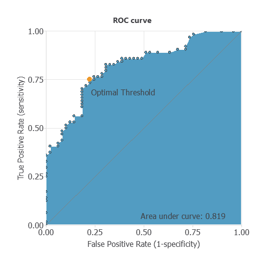
Final performance is calculated once on 113 rows assigned to the testing subset. At the fixed 0.50 threshold, the classifier detects 38 of 49 wilt-labelled segments and correctly rejects 47 of 64 other-land-cover segments.
| Actual / predicted | Wilt candidate | Other land cover | Total |
|---|---|---|---|
| Wilt | 38 | 11 | 49 |
| Other land cover | 17 | 47 | 64 |
| Total | 55 | 58 | 113 |
| Testing metric | Value | Operational reading |
|---|---|---|
| Accuracy | 75.2% | 85 of 113 testing segments are classified correctly |
| Wilt precision | 69.1% | 38 of 55 flagged segments are true positives in this split |
| Wilt sensitivity | 77.6% | 38 of 49 wilt-labelled segments are detected |
| Specificity | 73.4% | 47 of 64 other-land-cover segments are rejected |
| Wilt F1 | 0.731 | Harmonic balance of precision and sensitivity |
| Balanced accuracy | 75.5% | Mean of sensitivity and specificity |
| ROC AUC | 0.819 | Ranking performance across all score thresholds |
7. Inference and reproducibility
A defensible inference pipeline starts upstream of the neural network. Image segmentation and the five feature definitions must remain identical to the study pipeline, and every prediction must retain acquisition and segment identifiers for spatial review.
Illustrative threshold scenarios
The testing rows illustrate the operational trade-off. Lowering the cutoff prioritizes sensitivity and reduces missed wilt candidates, but sends more segments to review. These figures are retrospective; a real threshold must be chosen on separate validation data from the intended surveillance programme.
| Testing scenario | Threshold | Sensitivity | Specificity | False negatives | False positives | Interpretation |
|---|---|---|---|---|---|---|
| Nearest ROC corner | 0.51 | 77.6% | 75.0% | 11 | 16 | Balanced internal discrimination |
| Surveillance-first | 0.20 | 91.8% | 48.4% | 4 | 33 | Fewer missed candidates, substantially more field or image review |
Held-out calculation example
The rounded values below correspond to a row assigned to the testing subset. Its supplied target is other land cover. The exported model returns a wilt score of 0.020051 and therefore assigns the negative class at the 0.50 threshold.
| Input | Value |
|---|---|
glcm | 101 |
green | 190 |
red | 81 |
nir | 320 |
pan_band | 23 |
Try the exported tree-wilt classifier
Research demonstration. The calculation runs locally with the exact exported weights and preprocessing. Enter only features generated with the same segmentation and image-processing definitions. Values outside the validated domain are rejected.
Reproduce the calculation
The Python package contains the exact exported model, ordered input schema and executable example. The Neural Designer package contains the cleaned sample roles, initial and selected architectures, training settings and regenerated analyses.
8. Validity, uncertainty and limitations
- Derived sampling design. The tutorial table keeps all 500 source testing rows but adds only the 74 positive rows from the source training file. It excludes 4,265 negative training rows, then creates a new random split. The reported metrics are therefore not an evaluation on the official UCI test protocol.
- Outlier-selection boundary. Tukey thresholds are calculated before the model split and exclude seven negative rows. A confirmatory workflow should estimate cleaning thresholds from training data only and report sensitivity analyses with and without exclusions.
- Spatial dependence is untested. The table has no coordinates, acquisition blocks or segment-group identifiers. Random row splitting can place nearby or related image objects in different subsets.
- Image-processing contract is incomplete. The CSV does not package the pansharpening, segmentation, georeferencing or feature-extraction implementation needed to reproduce descriptors from raw imagery.
- Transfer is untested. Sensor calibration, illumination, season, atmospheric correction, geography, species mix and disease stage may shift the feature distributions.
- Training-curve warning. The initial run shows increasing selection error after its early minimum. Checkpointing at the best selection epoch and repeated grouped validation should precede any scientific conclusion.
- Uncalibrated decision score. The sigmoid output ranks candidates but is not demonstrated to be a calibrated probability. The 0.50 threshold has not been selected from surveillance costs.
- Endpoint boundary. A positive segment is a remote-sensing disease candidate, not laboratory confirmation of Japanese oak wilt, Japanese pine wilt or a causal organism.
References
- Johnson B. Wilt [Dataset]. UCI Machine Learning Repository; 2013. CC BY 4.0.
- Johnson BA, Tateishi R, Hoan NT. A hybrid pansharpening approach and multiscale object-based image analysis for mapping diseased pine and oak trees. International Journal of Remote Sensing. 2013;34(20):6969–6982.