In this example, we will build machine learning to estimate car emissions, a topical issue that should raise awareness in the reader.
Nowadays, it is essential to reduce CO2 emissions in the atmosphere to fight against climate change. Indeed, many laws forbid cars whose CO2 emissions are above a specific limit; they must be below it to be approved to drive through the roads. We will predict CO2 emissions with certain independent variables.
Any car company could adjust this value by modifying parameters like the engine’s size and many other engine features.For this study, we have gathered an extensive data set of different types of cars that could exist anywhere in the world.
This example is solved with Neural Designer. To follow it step by step, you can use the free trial.
Contents
1. Application type
2. Data set
The first step is to prepare the data set, which is the source of information for the approximation problem. It is composed of:
- Data source.
- Variables.
- Instances.
Data source
The file co2_emissions.csv contains the data for this example. Here, the number of variables (columns) is 12, and the number of instances (rows) is 7385.
Variables
In that way, this problem has the 12 following variables:
- make, car brand under study.
- model, the specific model of the car.
- vehicle_class, the car body type of the car.
- engine_size, size of the car engine, in Litres.
- cylinders, number of cylinders.
- transmission, “A” for ‘Automatic’, “AM” for ‘Automated manual’, “AS” for ‘Automatic with select shift’, “AV” for ‘Continuously variable’, and “M” for ‘Manual’.
- fuel_type, “X” for ‘Regular gasoline’, “Z” for ‘Premium gasoline’, “D” for ‘Diesel’, “E” for ‘Ethanol (E85)’, and “N” for ‘Natural gas’.
- fuel_consumption_city, City fuel consumption ratings, in liters per 100 kilometers.
- fuel_consumption_hwy, Highway fuel consumption ratings, in liters per 100 kilometers.
- fuel_consumption_comb(l/100km), the combined fuel consumption rating (55% city, 45% highway), in L/100 km.
- fuel_consumption_comb(mpg), the combined fuel consumption rating (55% city, 45% highway), in miles per gallon (mpg).
- co2_emissions, the tailpipe carbon dioxide emissions for combined city and highway driving, in grams per kilometer.
All the variables that appear in the study are inputs, except for ‘make’ and ‘model’, which have to stay “unused”, and ‘co2_emissions’, which is the output that we want to extract from this machine learning study.
Also, we realized that the instance ‘vehicle_class’ could be problematic to analyze because it contains many categorical variables inside. Still, in a further study, we can see that the final selection error is higher without this variable than including it.
Therefore, as one of the main goals of a Neural Network study is to minimize the Selection Error as much as possible, we can add ‘vehicle_class’ as an input.
As we can see, certain variables should stay “unused”, too. That is the case of ‘fuel_consumption’ (in city, highway, or combined). These instances could be targets of the study (CO2 and fuel consumption depend on each other), but it is more visual to see the CO2 emissions as the final output.
Instances
Instances are divided randomly into training, selection, and testing subsets containing 60%, 20%, and 20% of the instances. More specifically, 4431 samples are used here for training, 1477 for validation, and 1477 for testing.
Variables distribution
Once all the data set information has been set, we will perform some analytics to check the quality of the data.
For instance, we can calculate the data distribution. The next figure depicts the histogram for the target variable.
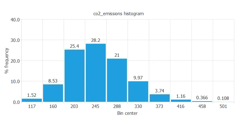
As we can see in the diagram, the CO2 emissions have a normal distribution. In fact, there are a lot of cars that have median CO2 emissions that stay below the limit we were talking about before. But, on the other hand, exactly 0.108 percent of the total cars in this study have very high CO2 emissions that nowadays would not be able to drive.
Inputs-targets correlations
The next figure depicts inputs-targets correlations. This might help us see the different inputs’ influence on the final car emissions.
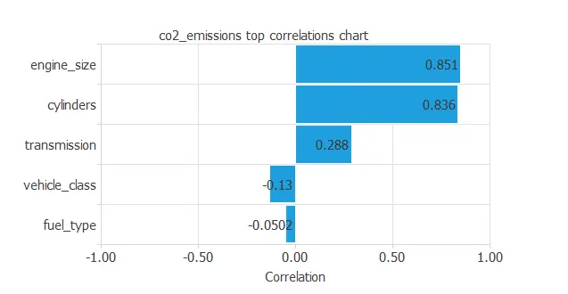
The above chart shows that a few instances depend on CO2 emissions. As we can see, “engine_size” and “cylinders” depend positively on CO2 emissions; the bigger the engine size, the more CO2 the car emits, for example. On the other hand, some instances have a negative dependency on the emissions.
Scatter charts
We can also plot a scatter chart with the CO2 emissions versus the engine size.
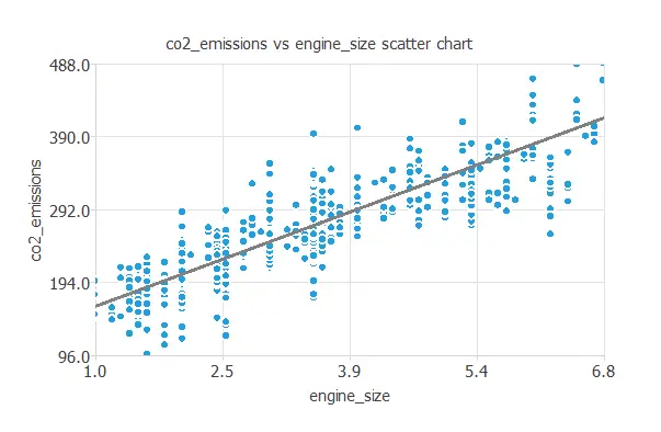
In general, the larger the engine size, the more emissions. However, CO2 emissions depend on all the inputs at the same time.
3. Neural network
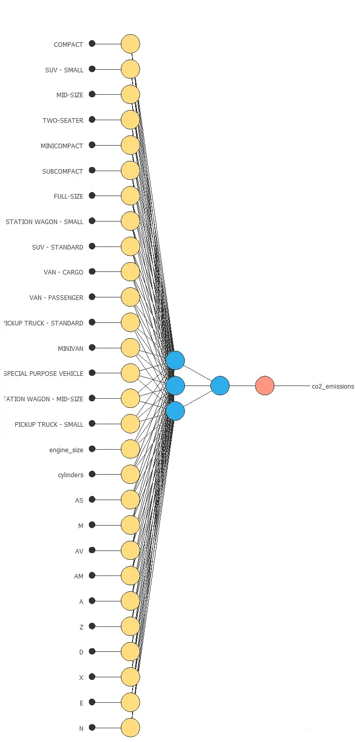
The neural network will output the CO2 emissions as a function of consumption, transmission, and other car engine features.
In this approximation example, the neural network comprises:
- Scaling layer.
- Perceptron layers.
- Unscaling layer.
Scaling layer
The scaling layer transforms the original inputs to normalized values. Here, the mean and standard deviation scaling method is set so that the input values have a mean of 0 and a standard deviation of 1.
Perceptron layers
Here, two perceptron layers are added to the neural network. Subsequently, this number of layers is deemed sufficient for most applications. Specifically, the first layer comprises 28 inputs and 3 neurons, while the second layer consists of 3 inputs and 1 neuron.
Unscaling layer
The unscaling layer transforms the normalized values from the neural network into the original outputs. Here, the mean and standard deviation unscaling method will also be used.
Network architecture
The next figure shows the resulting network architecture.
4. Training strategy
The next step is selecting an appropriate training strategy to define what the neural network will learn. A general training strategy is composed of two concepts:
- A loss index.
- An optimization algorithm.
Loss index
The loss index chosen is the normalized squared error with L2 regularization. This loss index is the default in approximation applications.
Optimization algorithm
The optimization algorithm chosen is the quasi-Newton method. This optimization algorithm is the default for medium-sized applications like this one.
Training process
Once we have set the strategy, we can train the neural network. The following chart shows how the training (blue) and selection (orange) errors decrease with the training epoch during the training process.
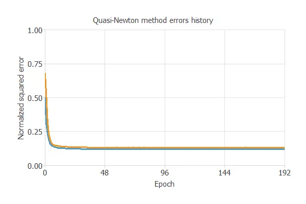
The most important training result is the final selection error. Indeed, this is a measure of the generalization capabilities of the neural network. Here, the final selection error is selection error = 0.145 NSE.
5. Model selection
The objective of model selection is to find the network architecture with the best generalization properties. We want to improve the final selection error obtained before (0.145 NSE).
The best selection error is achieved using a model whose complexity is the most appropriate to produce an adequate data fit. Order selection algorithms are responsible for finding the optimal number of perceptrons in the neural network.
The final selection error takes a minimum value at some point. Here, the optimal number of neurons is 10, corresponding to a selection error of 0.131.
6. Testing analysis
The objective of the testing analysis is to validate the generalization performance of the trained neural network. The testing compares the values provided by this technique to the observed values.
A standard testing technique in approximation problems involves performing a linear regression analysis between the predicted and the real values using an independent testing set. Consequently, the next figure illustrates a graphical output provided by this testing analysis.
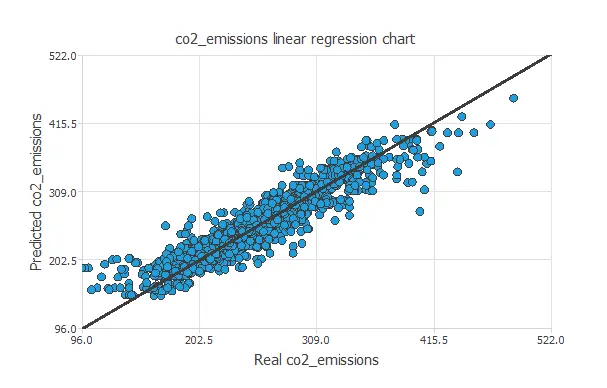
From the above chart, we can see that the neural network is predicting well the entire range of the CO2 emissions data. The correlation value is R2 = 0.924, which is close to 1.
7. Model deployment
The model is now ready to estimate the CO2 emissions of a certain car with satisfactory quality over the same data range.
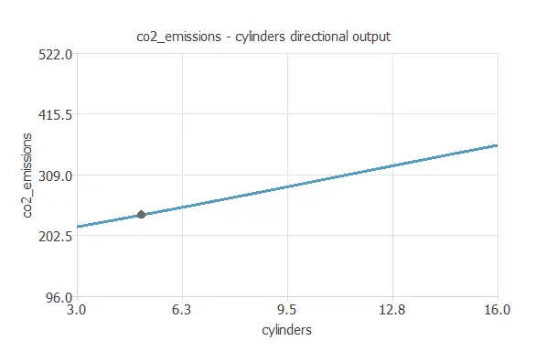
Directional output
We can plot a directional output of the neural network to see how the emissions vary with a given input for all other fixed inputs. The next plot shows the CO2 emissions as a function of the number of cylinders through the following point:
- vehicle_class: COMPACT.
- engine_size: 3.16 L.
- cylinders: 5.
- transmission: AS.
- fuel_type: Z.
Mathematical expression
The co2-emissions.py contains the Python code for the CO2 emissions.
References
- Kaggle Machine Learning Repository. CO2 Emissions by Vehicles Data Set.