Estimate vehicle price from specifications for market benchmarking
A compact neural network maps vehicle configuration, dimensions, powertrain and efficiency data to an indicative price. The model can support early product planning and portfolio benchmarking, while commercial decisions remain subject to current-market data and expert review.
1. Industrial challenge
Automotive product teams need an early view of how a proposed vehicle sits within a reference market before detailed costing, positioning and launch decisions are complete. This example builds an approximation model that estimates dataset price from 25 vehicle descriptors and exposes local sensitivity for specification reviews.
2. Data set
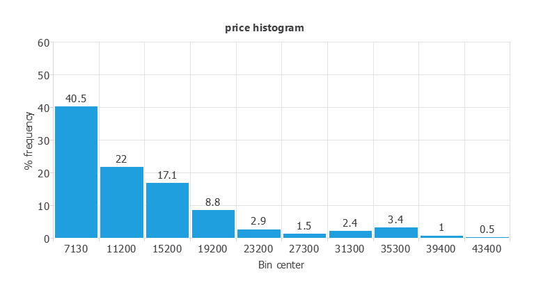
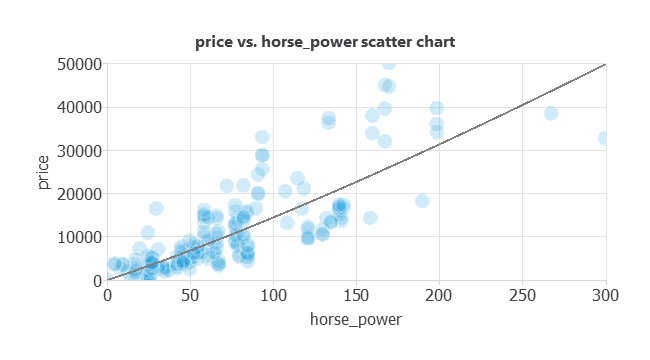
The dataset contains 205 vehicles and 27 columns: one identifier, 25 candidate inputs and the target price. car_id is excluded from modelling. Categorical variables are encoded by Neural Designer, so the 25 source inputs expand to 208 numerical features.
| Variable group | Fields | Role in the study |
|---|---|---|
| Market and configuration | symboling, car_brand, car_name, fuel, aspiration, doors, body, drive and engine location | Vehicle identity, risk rating and configuration |
| Dimensions and mass | Wheelbase, length, width, height and curb weight | Package size and vehicle mass |
| Powertrain | Engine type, cylinders, engine size, fuel system, bore, stroke, compression, horsepower and peak RPM | Mechanical specification and performance |
| Efficiency | City and highway MPG | Fuel-consumption indicators |
| Target | price | Dataset price in US dollars |
The configured random split assigns 123 rows to training, 41 to selection and 41 to testing. The published CSV has been byte-checked against the local dataset used to build the current project.
3. Model
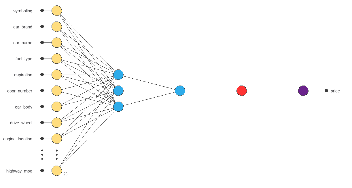
The model receives 25 source variables. Categorical expansion produces 208 numerical input features, which feed a dense hidden layer with three tanh neurons and a one-neuron identity output layer. Scaling is applied before the dense layers and the output is unscaled back to dollars.
4. Training strategy
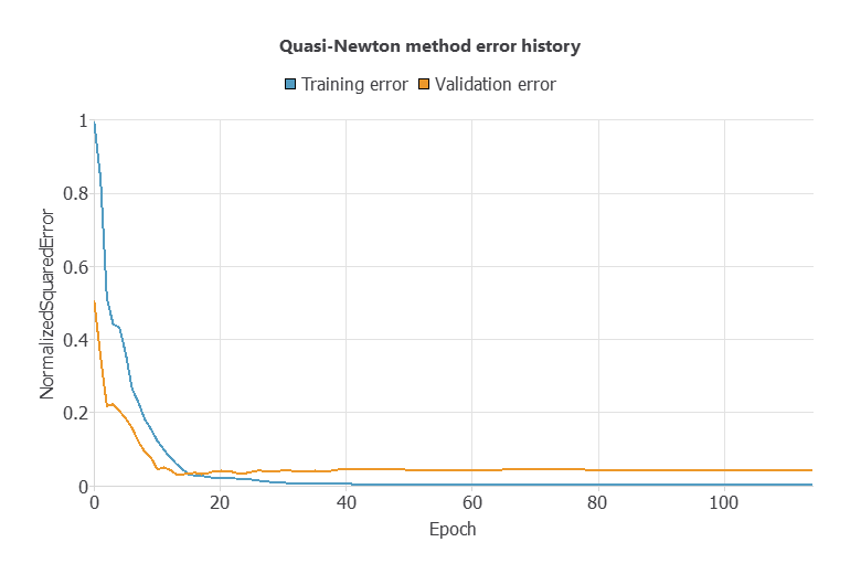
Training minimizes normalized squared error with L2 regularization (weight 0.01) using the quasi-Newton method. The latest run contains 114 completed epochs: training error ends at 0.00318, while selection error reaches a minimum of 0.0308 at epoch 14 and ends at 0.0426.
5. Model selection
No additional neuron-selection sweep was used for the updated model. The existing three-neuron hidden layer already provides a compact baseline with good selection and testing performance, so adding complexity would not be justified by the current evidence.
6. Testing analysis
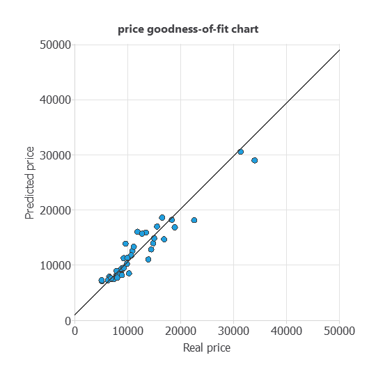
The independent testing subset contains 41 vehicles. The exported project gives a determination coefficient of 0.912; error metrics in dollars make the result easier to interpret operationally.
| Testing metric | Result | Interpretation |
|---|---|---|
| Testing vehicles | 41 | Independent rows in the configured random split |
| R² (determination) | 0.912 | Agreement between observed and predicted prices |
| R² (SSE definition) | 0.908 | Variance explained relative to the testing-set mean |
| Mean absolute error | $1,392 | Typical absolute pricing error |
| Root mean squared error | $1,881 | Gives more weight to large misses |
| 95th-percentile absolute error | $3,729 | Only about 5% of testing errors are larger |
| Maximum absolute error | $4,891 | Largest miss among the 41 testing vehicles |
7. Model deployment
In a professional workflow, the network would act as a specification-to-price surrogate. Its estimate should support product planning and market benchmarking, with input validation and analyst review rather than automatic price publication.
Representative specification review
The reference point used by Neural Designer is a Honda Civic CVCC configuration from the dataset. It is shown as an operational example, not as an independent validation case: the row belongs to the training subset.
| Input | Value |
|---|---|
| Insurance risk rating | 2 |
| Brand / model | Honda / Civic CVCC |
| Fuel / aspiration | Gas / standard |
| Doors / body | 2 / hatchback |
| Drive / engine location | Front-wheel drive / front |
| Wheelbase | 86.6 in |
| Length × width × height | 144.6 × 63.9 × 50.8 in |
| Curb weight | 1,819 lb |
| Engine type / cylinders | OHC / 4 |
| Input | Value |
|---|---|
| Engine size | 92 in³ |
| Fuel system | 1bbl |
| Bore × stroke | 2.91 × 3.41 in |
| Compression ratio | 9.2 |
| Horsepower | 76 hp |
| Peak engine speed | 6,000 rpm |
| City / highway economy | 31 / 38 mpg |
| Dataset price | $6,855 |
The model estimates $6,682, compared with the dataset value of $6,855. This close match demonstrates how the deployed calculation is read, but it must not be added to the testing performance because the row was used for training.
Engine-size sensitivity at the reference point
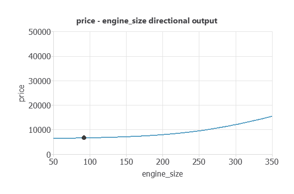
Holding all other fields fixed, the directional output increases from approximately $6,510 at 50 in³ to $15,500 at 350 in³. The grey point marks the 92 in³ reference configuration and its $6,682 prediction.
Integrate the exported model
The Python package contains input preprocessing, the trained 208–3–1 network and output unscaling. Its predict_vehicle() function accepts the original 25-field vehicle record and performs the categorical encoding internally. The repaired vector implementation was checked against the Neural Designer project; the maximum difference across the 41 testing rows was below $43, caused by the decimal precision of the generated Python weights.
8. Scope and limitations
- The dataset contains 205 vehicles and no transaction date, model year, inflation index, dealer incentive or regional market field; it is not a current-market pricing feed.
car_namehas 144 categories, and the complete categorical encoding expands 25 source variables to 208 features while only 123 rows are used for training. This creates a material overfitting risk.- The random row split does not prove transfer to unseen models or brands. In the configured testing subset, 24 of the 35 represented model-name levels do not appear in training.
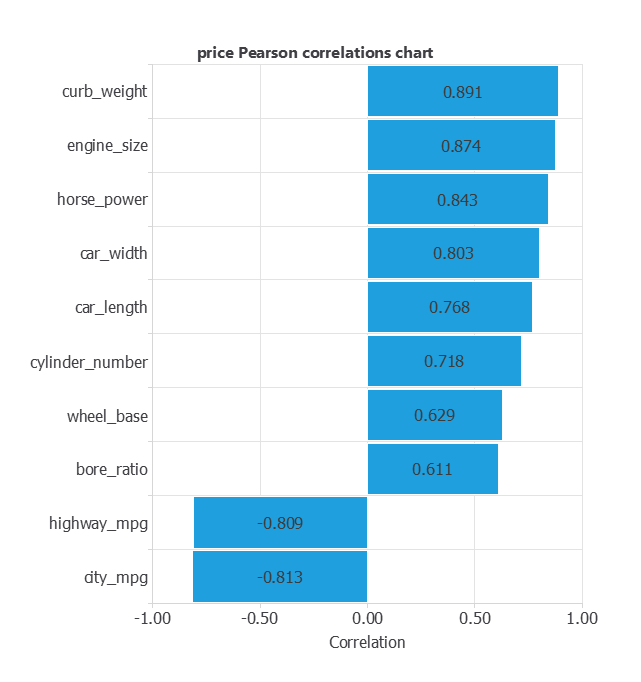
- Pearson correlations and one-variable directional outputs describe associations around this dataset; they are not causal estimates of the commercial value of an engineering change.
- Before production use, retrain on recent transactions or validated list prices, separate data by model family and time, compare against a transparent baseline and report prediction intervals.
- Deployment should reject unknown categories, monitor price and feature drift, retain model/version traceability and require commercial review for decisions outside the validated domain.