This tutorial describes different machine learning model types.
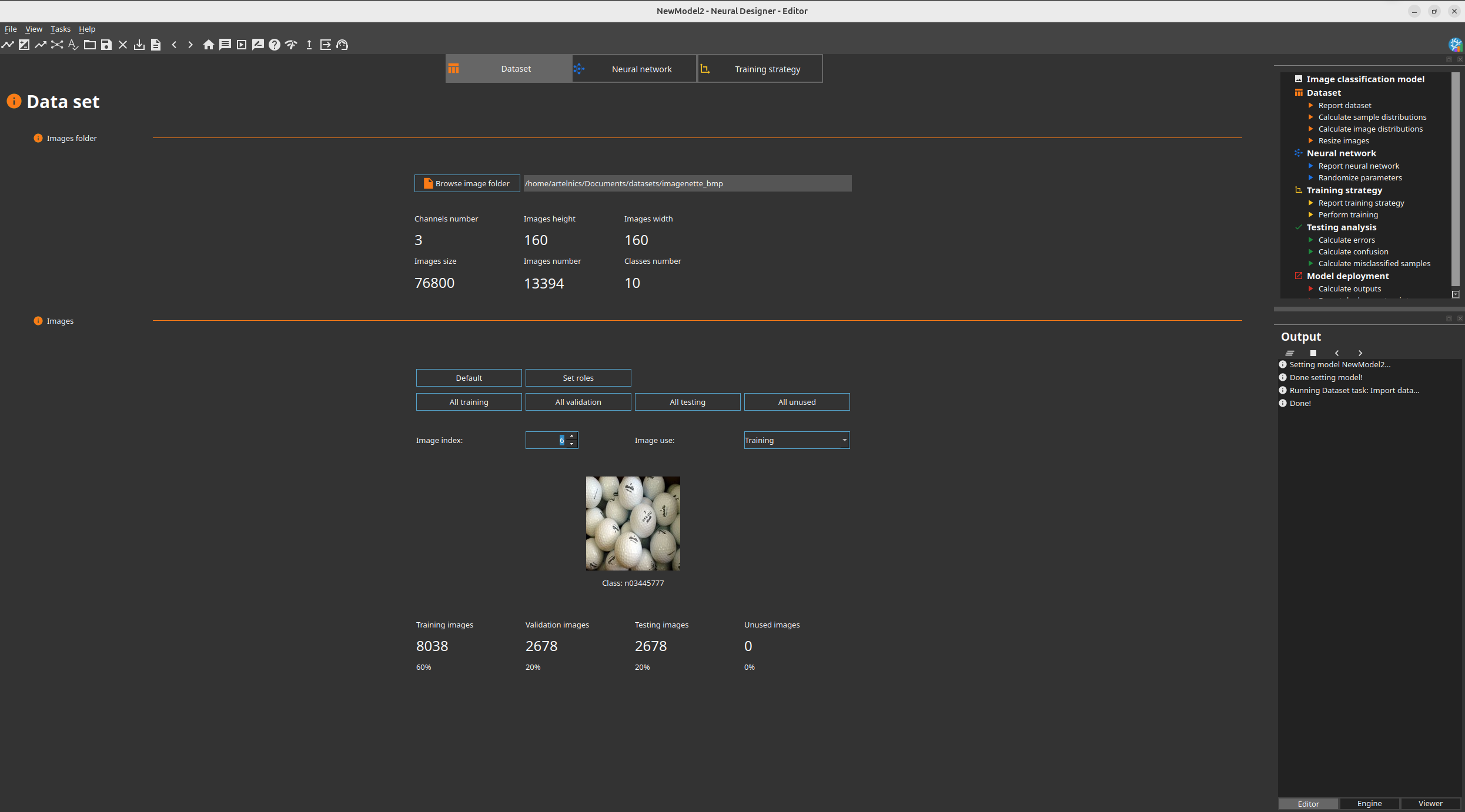
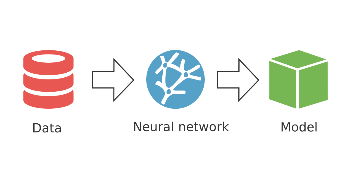
Neural networks use information in the form of data to generate knowledge in the form of models.
A model can be defined as a description of a real-world system or process using mathematical concepts.
It is usually represented as a mapping between input and output variables.
In this regard, neural networks are used to discover relationships, recognize patterns, predict trends, and recognize associations from data.
Model types
- 1.1. Approximation (or function regression)
- 1.2. Classification (or pattern recognition)
- 1.3. Forecasting (or time series prediction)
- 1.4. Anomaly detection
- 1.5. Text classification
- 1.6. Image classification model

1.1. Approximation (or function regression)
In an approximation problem, a neural network learns how one or more continuous target variables depend on a set of input variables. No formula for that relationship is available beforehand; the model has to infer it from examples.
The examples come from a data set. Each sample pairs the values of the input variables with the values measured for the target variables. During training, the targets play the role of the correct answers against which the outputs of the neural network are compared.
Once trained, the model returns an estimate of the targets for any new combination of inputs. In the simplest case there is a single input, x, and a single target, y, and the model is a curve that runs through the cloud of points, as the following figure shows.
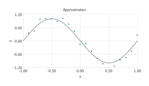
Approximation, also called regression, is one of the most widely used model types. Some examples are the following:
- Model the strength of high-performance concretes.
- Predict the noise generated by airfoil blades.
- Predict the residuary resistance of sailing yachts.
- Predict the electricity generated by combined cycle power plants.
- Forecast the power generated by a solar plant.
- Model wine preferences from physicochemical properties.
Measured targets are never exact. Each value combines a systematic part, which changes smoothly with the inputs, and a random part caused by sensor noise, unrecorded factors or rounding. In statistical terms, when errors are measured as squared differences, the best possible prediction for a given input is the mean of the target values that would be observed for it, and that mean is precisely the systematic part.
A good model therefore follows the trend and ignores the scatter around it. A neural network that bends to pass through every training point has also learned the noise, and its predictions for new samples get worse rather than better. The ability to predict well on samples that were not used for training is called generalization, and it is what ultimately decides how good an approximation model is. The Model selection chapter explains how to control it.

1.2. Classification (or pattern recognition)
A classification model assigns each sample to one category out of a fixed set. The inputs describe the sample, for example the measurements taken from a tumor or the activity of a customer, and the target records the category it belongs to.
Rather than returning a bare label, a neural network for classification estimates, for every class, the probability that the sample belongs to it given the values of its inputs. The predicted class is then the most probable one or, in binary problems, the one chosen by a decision threshold. Probabilities say more than labels: they show how confident the model is, and they let you balance false positives against false negatives.
In the following figure, each sample is described by two inputs, x1 and x2, and belongs to one of two classes, drawn as circles and green squares. The model has to find a boundary that separates the two groups.
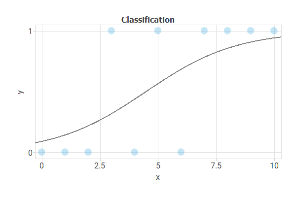
As in approximation, what counts is the performance on samples that the model has not seen: a boundary that wraps tightly around every training point usually classifies new data worse than a smoother one.
We can distinguish between two types of classification models:
Binary classification
In binary classification, the target variable is usually binary (true or false).
Some examples are to:
- Diagnose breast cancer from fine-needle aspirate images.
- Reduce employee attrition.
- Increase the conversion rate of telemarketing campaigns in banks.
- Predict the probability of default of credit card clients.
- Detect diseased trees from remote sensing data.
- Target donors in blood donation campaigns.
- Diagnose acute inflammations of the urinary bladder.
- Predict customer churn in telecommunications companies.
Multiple classification
In multiple classifications, the target variable is usually nominal (class_1, class_2, or class_3).
Some examples are the following:

1.3. Forecasting (or time series prediction)
A forecasting model predicts the values that one or more variables will take in the future, using the values that they, and possibly other variables, took in the past.
The data come as a time series: observations recorded at regular intervals, such as every hour, day or month. To train a neural network, the series is rearranged into samples. In Neural Designer, you choose the number of lags and the number of steps ahead: the inputs of each sample are the observations at the current time step and at the previous ones (the lags), and the targets are the values at the following time steps. After this rearrangement, a forecasting model is trained much like an approximation model.
The following figure illustrates a forecast application: the model estimates the next value, yt+1, from the current value, yt, the previous one, yt-1, and so on.
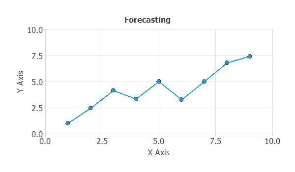
For instance, a car manufacturer can forecast next month’s sales of a model from its sales in previous months, its recent marketing actions and macroeconomic indicators.
A forecasting model is only useful if its predictions hold beyond the period it was trained on. For that reason, it is good practice to test it on the most recent part of the series, which the model has not seen during training.

1.4. Anomaly detection
Anomaly detection identifies samples that depart from normal behavior. In Neural Designer, this model uses an auto-associative neural network to reconstruct its own input variables. It learns from normal training samples; it does not need a separate target variable for training.
The following figure illustrates the reconstruction network used by the model:
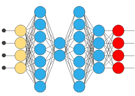
The difference between a sample and its reconstruction is an error score. Samples whose score reaches or exceeds the anomaly threshold are flagged for review. Neural Designer can calculate a threshold from normal training errors or use a threshold chosen by the user.
Typical applications include spotting unusual sensor readings in industrial equipment, abnormal ECG measurements, and deviations in process or environmental data.
Prepare normal samples for training and reserve separate samples for testing. An optional Evaluation variable can hold known labels (0 for normal, 1 for anomalous); it stays out of the model and is used only to assess detection results.
For this model, Neural Designer provides tasks to inspect sample reconstructions, calculate anomaly thresholds, evaluate detection tests and ROC curves when labels are available, detect anomalies in a new CSV file, and export an anomaly detector.
Explore three Anomaly Detection examples with saved task results:
- ECG anomaly detection — Research benchmark on ECG5000 beat classes from one recording.
- Bearing anomaly detection — Four-bearing vibration feature review.
- Hydraulic system anomaly detection — Hydraulic cycle monitoring with a training-derived threshold.

1.5. Text classification
Text classification is a natural language processing task in which text data is categorized into predefined labels or categories.
The basic goal of a text classification problem is to model one or several target variables conditioned on the input text data.
The objective here is to predict the category or label of a given text based on its content.
In text classification applications, the targets are usually discrete variables such as categories, labels, or sentiments.
Some examples are the following:
- Spam detection: Classifying emails as spam or not based on their content.
- Sentiment analysis: Classifying text data as positive, negative, or neutral based on the sentiment expressed.
- Topic classification: Classifying news articles into predefined topics such as politics, sports, technology, etc.
- Named entity recognition: Identifying and classifying named entities such as people, organizations, locations, etc.
Text data are noisy in their own way. Typos, grammatical errors, abbreviations and passages unrelated to the label add variation that says nothing about the category, while the useful information lies in recurring words, phrases and patterns.
The aim is a model that relies on those recurring patterns rather than on accidental details of the training documents, so that it also assigns the right category to texts it has never seen.

1.6. Image classification model
Image classification is a computer vision task in which an entire image is assigned to one of a predefined set of classes. Unlike a conventional classification data set, every input sample is a three-dimensional tensor of pixel values with the shape height × width × channels. The model learns the visual features that distinguish one class from another directly from those pixels.
In Neural Designer, an image classification project combines an image data set with a convolutional neural network. Images are organized into one folder per class, and the folder names define the class labels. The data set must contain at least two non-empty class folders.
The image classification model processes the data through the following architecture:
- Image scaling: Pixel values are normalized with image min-max scaling.
- Feature extraction: One or more 3 × 3 convolutional layers with ReLU activation learn local visual patterns. Each convolutional block is followed by 2 × 2 max pooling.
- Classification: The extracted feature maps are flattened and passed to a dense ReLU layer.
- Output: Binary problems use a sigmoid output, while multiclass problems use a softmax output.
Cross-entropy is the appropriate loss for this task, and adaptive moment estimation is commonly used to train the network. The trained model can be evaluated with a confusion matrix and the corresponding binary or multiclass classification metrics.
Typical applications include handwritten character recognition, medical image classification, visual quality inspection, remote-sensing image analysis, and species or disease identification from photographs.