Introduction
Machine learning models for blood donation prediction can help healthcare organizations improve donor recruitment and optimize campaigns.
Since reaching donors remains a challenge, a neural network trained on features such as recency, frequency, and time since the first donation.
Using data from the Blood Transfusion Service Center in Hsin-Chu City, Taiwan, the model achieved an AUC of 0.714 and 63.8% of accuracy, demonstrating strong potential as a predictive support tool for donor behavior.
Healthcare professionals can test this methodology by downloading Neural Designer.
Contents
The following index outlines the steps for performing the analysis.
1. Model type
- Problem type: Binary classification (blood donor or non-donor)
- Goal: Model the probability of donating blood based on individual features to support decision-making using artificial intelligence and machine learning.
2. Data set
Data source
The blood_donation.csv dataset contains 748 instances and 4 variables used to build the model.
Variables
The following list summarizes the variables’ information:
Donor history
recency (months) – Months since the last donation.
time (months) – Months since the first donation.
Donation behavior
frequency (count) – Total number of donations.
Target variable
- donation (yes or no) – Did the person donate in the last campaign?
Instances
The dataset’s instances are split into training (60%), validation (20%), and testing (20%) subsets by default.
You can adjust them as needed.
Variables distribution
Variable distributions can be calculated; the figure shows the number of donations (1) versus non-donations (0) in the dataset.
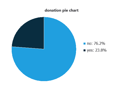
As depicted in the image, donations represent 76.2% of the samples, and no donations represent approximately 23.8%.
Input-target correlations
The input-target correlations indicate which factors most influence whether a person would donate blood and, therefore, are more relevant to our analysis.
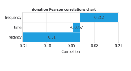
Here, the most correlated variables with blood donation are recency and frequency.
3. Neural network
A neural network, inspired by the human brain, takes input variables and outputs the probability of blood donation.
Trained on historical data, the network learns patterns that support decision-making.
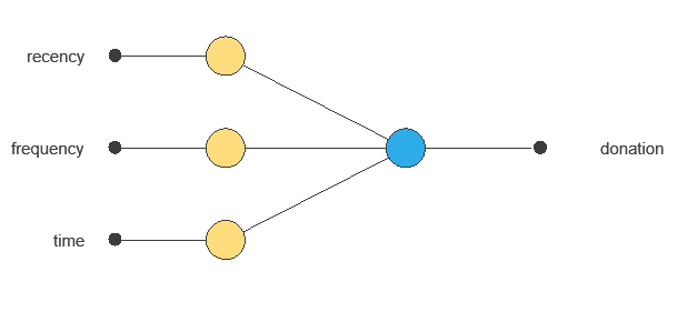
The network uses three donor variables to output the probability of blood donation, with connections showing each variable’s contribution.
4. Training strategy
Training a neural network uses a loss function to measure errors and an optimization algorithm to adjust the model, ensuring it learns from data while generalizing well to new cases.
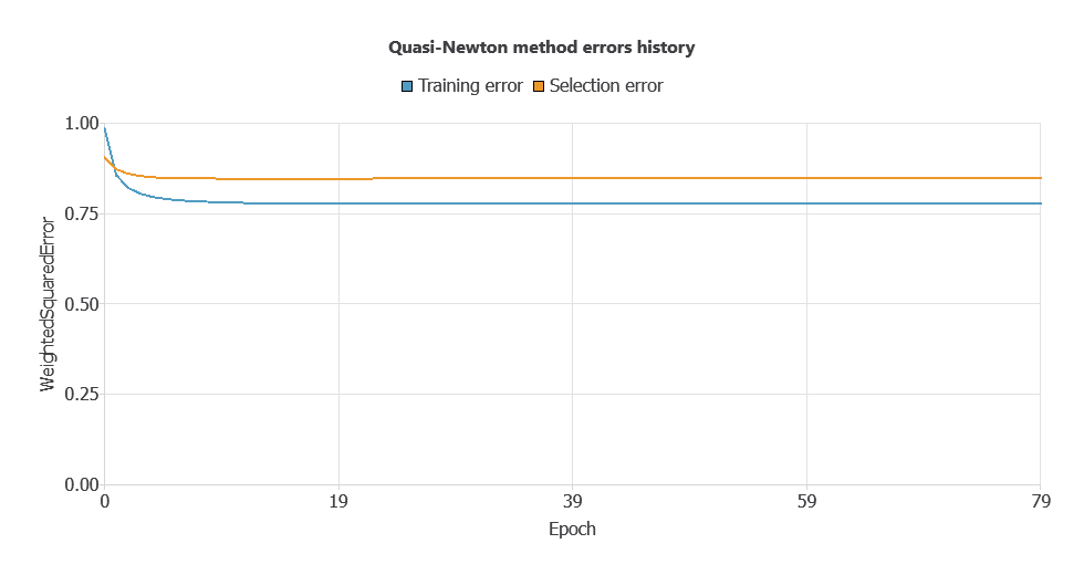
The model trained stably on new data, with steadily decreasing training and selection errors (0.777 and 0.847).
5. Testing analysis
The objective of the testing analysis is to validate the performance of the trained neural network.
ROC curve
The ROC curve is a standard tool to evaluate a classification model, showing how well it distinguishes between two classes by comparing predicted results with actual outcomes.
A random classifier scores 0.5, while a perfect classifier scores 1.
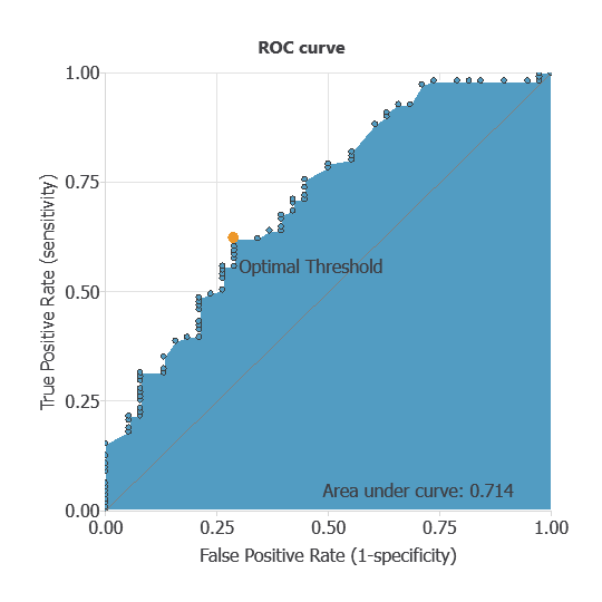
The AUC obtained is 0.714, showing that the model performs well at distinguishing between donors and non-donors.
Confusion matrix
The confusion matrix evaluates the model’s performance by comparing predicted and actual outcomes:
True positives: donors correctly classified as donors.
False positives: non-donors incorrectly classified as donors.
False negatives: donors incorrectly classified as non-donors.
True negatives: non-donors correctly classified as non-donors.
For a decision threshold of 0.5, the confusion matrix was:
| Predicted positive | Predicted negative | |
|---|---|---|
| Real positive | 27 | 11 |
| Real negative | 46 | 65 |
In this case, 61.74% of cases were correctly classified and 38.26% were misclassified.
Binary classification
The performance of this binary classification model is summarized with standard measures:
Accuracy: 63.8% of cases were correctly classified.
Error rate: 36.2% of cases were misclassified.
Sensitivity: 63.2% of donors were correctly identified.
Specificity: 64% of non-donors were correctly identified.
The model performs moderately at detecting donors and better at identifying non-donors.
6. Model deployment
After confirming the neural network’s ability to generalize, the model can be saved for future use in deployment mode.
This allows the trained network to be applied to new individuals, using their clinical and demographic variables to calculate the probability that a person will donate blood.
In deployment mode, healthcare professionals can use the model as a reliable diagnostic support tool for classifying new patients.
The Neural Designer software exports the trained model automatically, making it easy to integrate into clinical practice.
Conclusions
The blood donation prediction model achieved an AUC of 0.714 and 63.8% of accuracy.
Recency, frequency, and time since first donation were the most influential features, reflecting known donor behavior.
This neural network can support healthcare organizations in identifying potential donors and improving recruitment efficiency.
References
- The data for this problem has been taken from the UCI Machine Learning Repository.
- Yeh, I-Cheng, Yang, King-Jang, and Ting, Tao-Ming, “Knowledge discovery on RFM model using Bernoulli sequence“, Expert Systems with Applications, 2008.