This example assesses the death risk of patients who experienced heart failure.
Cardiovascular diseases are the leading cause of death worldwide, often leading to heart failure.
Using clinical data from 299 patients, this dataset with 12 features can help predict mortality.
A machine learning model can support early detection and improve patient management.
The data was collected by the Institutional Review Board of Government College University, Faisalabad (Pakistan), and is available in the Plos One Repository.
Also, we use the data science and machine learning platform Neural Designer to build the model. You can follow this example step by step using the free trial.
Contents
- Application type.
- Data set.
- Neural network.
- Training strategy.
- Model selection.
- Testing analysis.
- Model deployment.
1. Application type
2. Data set
Data source
The heart_failure.csv file contains the data for this example. Target variables can only have two values in a classification model: 0 (false, alive) or 1 (true, deceased), depending on the event’s occurrence. The number of patients (rows) in the data set is 299, and the number of variables (columns) is 12.
Variables
The following list summarizes the variables’ information:
Patient information
age – Age of the patient.
sex – Woman or man.
smoking – 1 if the patient smokes, 0 otherwise.
diabetes – 1 if the patient has diabetes, 0 otherwise.
high_blood_pressure – 1 if the patient has hypertension, 0 otherwise.
anaemia – Low red blood cell or hemoglobin count.
Clinical measurements
creatinine_phosphokinase – Level of CPK enzyme in the blood.
ejection_fraction – Percentage of blood pumped out with each heartbeat.
platelets – Platelet count in the blood.
serum_creatinine – Creatinine level in the blood.
serum_sodium – Sodium level in the blood.
Target variable
- death_event – 1 if the patient died during follow-up, 0 otherwise.
The number of input variables, or attributes for each sample, is 11.
The target variable is 1, death_event (1 or 0), indicating whether the patient has died or survived.
Instances
Variables distributions
Also, we can calculate the distributions for all variables. The following figure is a pie chart showing which patients are dead (1) or alive (0) in the data set.

The image shows that dead patients represent 32.107% of the samples, while live patients represent 67.893%.
Inputs-targets correlations
The inputs-targets correlations might indicate which factors have the most univariate influence on whether or not a patient will live.
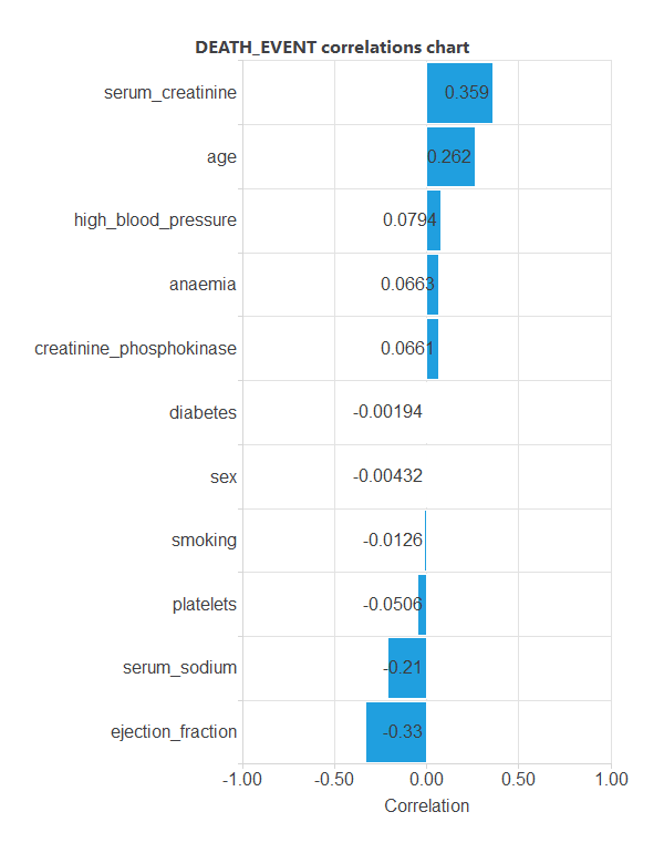
Here, the most correlated variables with survival status are serum_creatinine, age, serum_sodium, and ejection_fraction.
3. Neural network
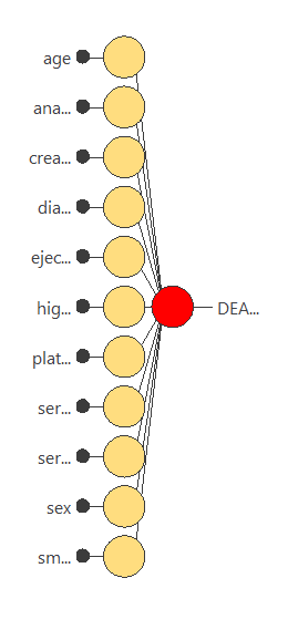
The next step is to set up a neural network representing the classification function. For this class of applications, the neural network is composed of:
The scaling layer contains the statistics on the inputs calculated from the data file and the method for scaling the input variables. Here, the minimum-maximum method has been set. As we use 11 input variables, the scaling layer has 11 inputs.
We won’t use a perceptron layer to stabilize and simplify our model.
The probabilistic layer only contains the method for interpreting the outputs as probabilities. Moreover, as the output layer’s activation function is logistic, that output can already be interpreted as a probability of class membership.
The probabilistic layer has 11 inputs. It has one output, representing the probability of a patient being dead or alive.
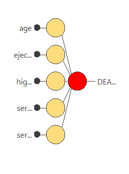
The following figure is a graphical representation of this neural network.
4. Training strategy
The fourth step is to set the training strategy, which is composed of two terms:
- A loss index.
- An optimization algorithm.
The loss index is the weighted squared error with L2 regularization, the default loss index for binary classification applications.
We can state the learning problem as finding a neural network that minimizes the loss index. That is a neural network that fits the data set (error term) and does not oscillate (regularization term).
The optimization algorithm that we use is the quasi-Newton method, which is also the standard optimization algorithm for this type of problem.
The following chart shows how errors decrease with the iterations during training.
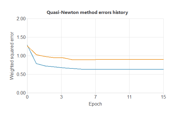
The final errors are 0.632 WSE for training and 0.899 WSE for selection.
The curves have converged, but since the selection error is higher, the model could still be improved to further reduce errors.
5. Model selection
The objective of model selection is to find the network architecture that minimizes the error, that is, with the best generalization properties for the selected instances of the data set.
Order selection algorithms train several network architectures with different numbers of neurons and select that with the smallest selection error. We have removed our perceptron layer to stabilize our model, so we cannot use this feature.
However, we will use input selection to select features in the data set that provide the best generalization capabilities.
The following image shows the training and selection errors as a function of the number of inputs using this method.
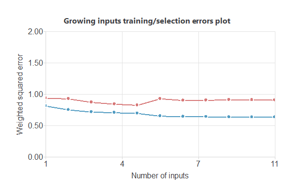
In the end, we obtain a training error = 0.693 WSE and a selection error = 0.823 WSE, respectively. Also, we have reduced the number of inputs to only 5 features. Our network is now like this:
6. Testing analysis
The objective of testing analysis is to validate the generalization performance of the trained neural network. To validate a classification technique, we need to compare the values provided by this technique to the observed values.
We can use the ROC curve as it is the standard testing method for binary classification projects.
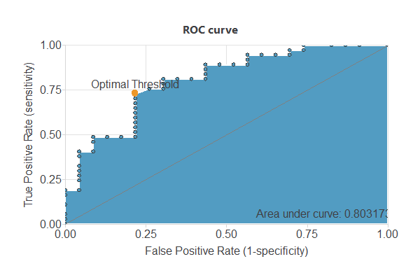
A random classifier has an AUC of 0.5, while a perfect one reaches 1. With an AUC of 0.803, this model shows good performance.
The following table shows the confusion matrix, including true positives, false positives, false negatives, and true negatives for the variable diagnosis.
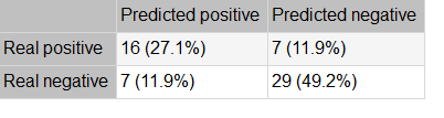
The binary classification tests are parameters for measuring the performance of a classification problem with two classes:
- Accuracy (ratio of instances correctly classified): 0.762
- Error (ratio of instances misclassified): 0.237
- Specificity (ratio of real positives that the model predicts as positives): 0.805
- Sensitivity (ratio of real negatives that the model predicts as negatives): 0.695
7. Model deployment
Once we have tested the neural network’s generalization performance, we can save it for future use in the so-called model deployment mode.
References
- The data for this problem has been collected by the Institutional Review Board of Government College University, Faisalabad-Pakistan, available at Plos One Repository.