Introduction
This application uses machine learning to assist health professionals in identifying renal pelvis nephritis, providing a presumptive diagnosis to complement expert evaluation.
Renal pelvis nephritis is relatively common and can be difficult to diagnose early, as symptoms often overlap with other renal conditions.
Our neural network model analyzes patient symptom data from the dataset to predict acute renal pelvis nephritis.
This approach offers healthcare professionals an additional tool to support diagnostic decision-making and improve patient care.
Healthcare professionals can test this methodology by downloading Neural Designer
Contents
The following index outlines the steps for performing the analysis.
1. Model type
Problem type: Binary classification (presence or absence of urinary disease)
Goal: Model the probability of renal pelvis nephritis based on patient features and diagnostic test results to support clinical decision-making
2. Data set
Data source
The dataset contains 120 instances and 7 variables for this example.
Variables
The dataset contains 6 input variables representing patients’ symptoms, as well as the target variable.
Patient variables
temperature (°C) – The patient’s body temperature.
nausea (yes or no) – Indicates if the patient feels nauseated while urinating.
lumbar_pain (yes or no) – Lumbar pain while urinating.
urine_pushing (yes or no) – Urgent need to urinate even when the bladder is empty.
micturition_pain (yes or no) – Pain during urination.
burning_of_urethra (yes or no) – Burning sensation while urinating.
Target
- nephritis of renal pelvis origin (yes or no) – Indicates renal pelvis nephritis.
Instances
The dataset’s instances are split into training (60%), validation (20%), and testing (20%) subsets by default.
You can adjust them as needed.
Variables distributions
Variable distributions can be examined; the figure shows a pie chart of positive and negative cases of renal pelvis nephritis in the dataset.
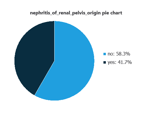
As depicted in the image, positive cases of nephritis of renal pelvis origin represent 41% of the samples, while negative cases represent 58%.
Input-target correlations
The input-target correlations indicate which factors most influence whether a patient has nephritis of renal pelvis origin and, therefore, are more relevant to our analysis.
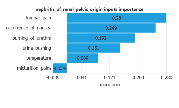
Here, the most correlated variables with malignant tumors are lumbar pain, occurrence of nausea, and burning of urethra.
3. Neural network
A neural network is an artificial intelligence model inspired by how the human brain processes information.
It is organized in layers: the input layer receives the variables, and the output layer provides the probability of belonging to a given class.
The network learns patterns fr style=”text-align: justify;”om historical data to predict nephritis, providing objective support for clinical decision-making.
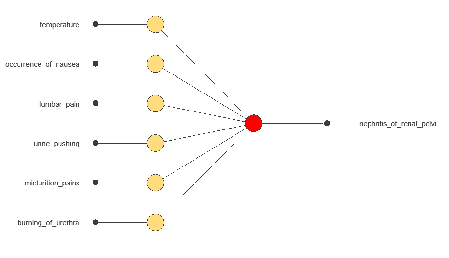
The network processes six diagnostic variables and produces a single output: the probability of developing nephritis of renal pelvis origin.
4. Training strategy
Training a neural network involves using a loss function and an optimization algorithm to learn from data while avoiding overfitting, ensuring good performance on new cases.
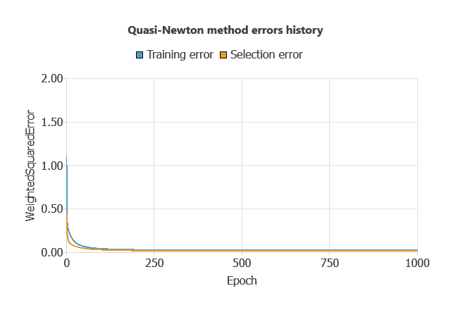
The model was trained to minimize errors while avoiding overfitting, achieving steady training and selection errors (0.023 and 0.016).
5. Testing analysis
An exhaustive testing analysis is performed to validate the generalization performance of the trained neural network.
ROC curve
The ROC curve evaluates the model’s ability to distinguish between patients with and without nephritis.
A random classifier scores 0.5, while a perfect classifier scores 1.
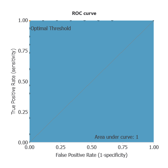
The AUC obtained is of 1, showing that the model performs perfectly at distinguishing between patients with and without renal pelvis nephritis.
Confusion matrix
The confusion matrix shows the model’s performance by comparing predicted and actual diagnoses. It includes:
True positives: patients correctly identified as having renal pelvis nephritis
False positives: patients incorrectly identified as having nephritis
False negatives: patients with nephritis incorrectly identified as not having it
True negatives: patients correctly identified as not having nephritis
For a decision threshold of 0.5, the confusion matrix was:
| Predicted positive | Predicted negative | |
|---|---|---|
| Real positive | 9 | 0 |
| Real negative | 0 | 15 |
In this case, 100% of cases were correctly classified and 0% were misclassified.
Binary classification
The performance of this binary classification model is summarized with standard measures:
Accuracy: 100% of patients were correctly classified.
Error rate: 0% of cases were misclassified.
Sensitivity: 100% of patients with nephritis were correctly identified.
Specificity: 100% of patients without nephritis were correctly identified.
These measures indicate that the model is highly effective at distinguishing between patients with and without renal pelvis nephritis.
6. Model deployment
After confirming the neural network’s ability to generalize, the model can be saved for future use in deployment mode.
This allows the trained network to be applied to new patients, using their clinical variables to calculate the probability of having renal pelvis nephritis.
In deployment mode, healthcare professionals can use the model as a reliable diagnostic support tool for classifying new patients.
The software exports the trained model automatically, making it easy to integrate into clinical practice.
Conclusions
The renal pelvis nephritis diagnostic model, built with the dataset, showed outstanding performance (AUC = 1, accuracy = 100%).
The most relevant features—lumbar pain, nausea, and burning urination—match established clinical knowledge, confirming its reliability.
With strong generalization to new patients, this approach can support healthcare professionals by providing presumptive diagnoses that complement expert evaluation and improve decision-making.
References
- UCI Machine Learning Repository.Acute inflammations data set.
- J.Czerniak, H.Zarzycki, Application of rough sets in the presumptive diagnosis of urinary system diseases, Artificial Intelligence and Security in Computing Systems, ACS’2002 9th International Conference Proceedings, Kluwer Academic Publishers,2003, pp. 41-51.