To build the model, we use data collected by the Cervical Pathology Unit in the health area of Palencia (Spain) from women participating in a cervical cancer early detection program.

2. Application type

The variable to be predicted is continuous (PROGNOSIS). Therefore, this is an approximation project.
The basic goal of this study is to model the patient’s prognosis as a function of the input variables.

3. Data set

The data set contains the relevant information to create the prognostic model.

Data source

In this case, the cervixcancer.csv contains the information for this study. Each column represents a variable related to cervical cancer, and each row represents a patient from the Cervical Pathology Unit.

Variables

The number of variables is 7, corresponding to the different tests for each patient. The number of cases is 197, the patients of the last three years with a definitive diagnosis. The following table shows the first 10 cases of this data set. We can observe that some missing values are represented by “NA”.

Neural networks work with numerical values. However, some of the variables in the table above have categorical values. Therefore, the first step is to assign numerical values to all categorical variables.

Age

The age is a numerical value that indicates the age of the patients. The variable AGE is numeric; therefore, it is unnecessary to modify it.

Cytology

Cytology is the primary tool for the prevention of cervical cancer. It is a diagnostic test based on the morphological study of cells. It is obtained by scraping or brushing the surface of the exocervix and endocervix, and it detects cervical cancer precursor lesions, which are ASC-US, ASC-H, L-SIL, H-SIL, and AGC. The variable CYTOLOGY contains NORMAL, ASC-US, ASC-H, L-SIL, H-SIL, and AGC values. This variable is ordinal since its values are different degrees of the same manifestation, and we can order them by severity. The following table shows the numerical values assigned to the results of this test.

HPV

Human papillomavirus. The HPV variable contains NEGATIVE, HPV 16, HPV 18, OTHER LOW RISK, and OTHER HIGH RISK. This variable is also considered ordinal. HPV 16 and HPV 18 represent the same risk, the maximum. The following table shows the numerical values assigned to the results of this test.

Biopsy

A test for a histological diagnosis of intraepithelial lesions and cervical cancer. It classifies the results as:

• CIN I: Mild dysplasia.
• CIN II: Moderate dysplasia.
• CIN III: Severe dysplasia and carcinoma in situ.

The variable BIOPSY has the values NOT ACCURATE, NEGATIVE, CIN I, CIN II-III, CIN III, and CARCINOMA. The biopsy is also an ordinal variable. The following table represents the grade assigned to each of these values.

P16/KI67:

Smoke

Variable indicating whether the patient is a smoker or not. The variable SMOKE is also binary. The value YES is assigned the number 1, and NO is assigned the number 0, as shown in the following table.

Prognosis

This is the variable that we want to predict. After testing, it indicates the absence of illness or the degree of disease. The prognosis values are NEGATIVE, CIN I, CIN II, CIN II-III, CIN III, ADENOCARCINOMA, AND SQUAMOUS CA. This variable is also ordinal. The following table shows the grade assigned to each of these values.

Once we have assigned numerical values to all ordinal and binary variables, we have a data set ready to be modeled by a neural network.
The following table shows the first 10 cases of this transformed data set.

The variables are of two types:

• Input variables: these are the predictors of the model (age, cytology, HPV, biopsy, p16/ki67, and smoke).
• Target variables: these are the variables to be predicted (PROGNOSIS).

The following chart illustrates the use of the variables. As we can see, our data set has six input variables and one target variable.

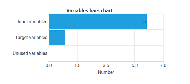
Instances

On the other hand, cases can be of three types:

• Training cases are used to build different prognostic models with different topologies.
• Selection cases are used to select the prognostic model with the best predictive capabilities.
• Test cases are used to validate the performance of the prognostic model.

The following pie chart details the uses of all cases in the data set.

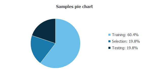
There are 119 training cases (60.4%), 39 generalization cases (19.8%), and 39 validation cases (19.8%).

Statistics

The bare statistics provide valuable information when designing a model since they tell us the variables’ ranges.
The table below shows the minimums, maximums, means, and standard deviations of all variables in our data set.

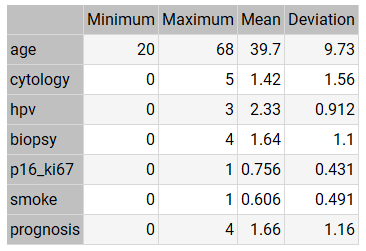
As we can see from the statistics:

• The mean AGE of the patients is around 40 years.
• The mean CYTOLOGY value is low (between ASC-US and ASC-H).
• The mean HPV value is high (between OTHER HIGH RISK and HPV 16-18).
• The mean value of BIOPSY is neither high nor low (between CIN I and CIN II).
• The mean value of P16/KI67 is very high.
• The mean value of SMOKE is high.
• The mean value of PROGNOSIS is neither high nor low (between CIN I and CIN II).

The mean PROGNOSIS value (1.66) is slightly higher than the mean BIOPSY value (1.64). This indicates that the mean evolution of patients tends to be stable, although it tends to worsen.

Distributions

Histograms and pie charts show the distribution of the data over their entire range. A uniform or Gaussian distribution of all variables is generally desirable for predictive analysis. Conversely, if the data is uneven, the model will likely be poor quality.

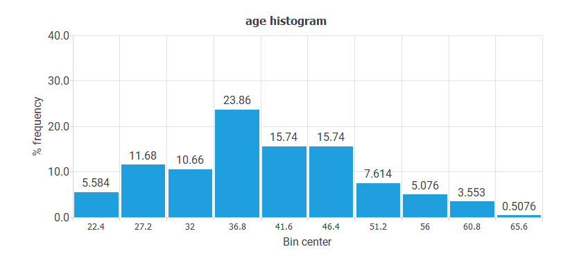
• The following chart shows the histogram for the variable AGE. The abscissa represents the midpoints of the rectangles, and the ordinate represents their corresponding frequencies. This distribution is Gaussian, and the center is at 36.8.
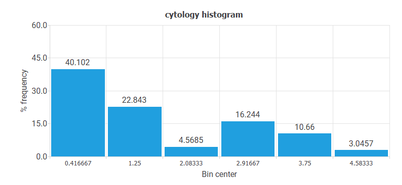
• The following chart shows the histogram for the variable CYTOLOGY. The majority of values correspond to the NORMAL value. The least represented values are ASC-H and AGC.
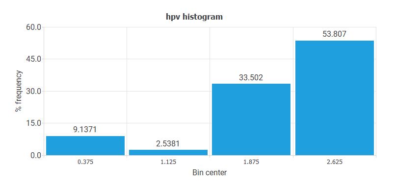
• The following chart shows the histogram for the HPV variable. Here, the majority of cases have HPV 16 or HPV 18 values. The least represented patients are OTHER LOW RISK.
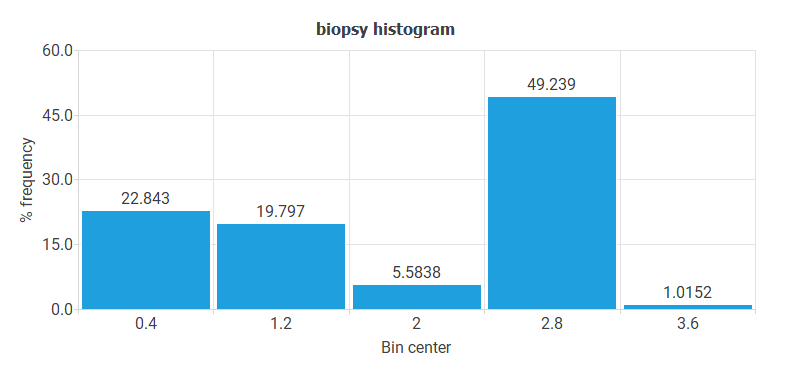
• The following chart shows the histogram for the variable BIOPSY. These data do not have a regular distribution. Indeed, most cases have CIN II-III or CIN III, and very few cases have ADENOCARCINOMA value.
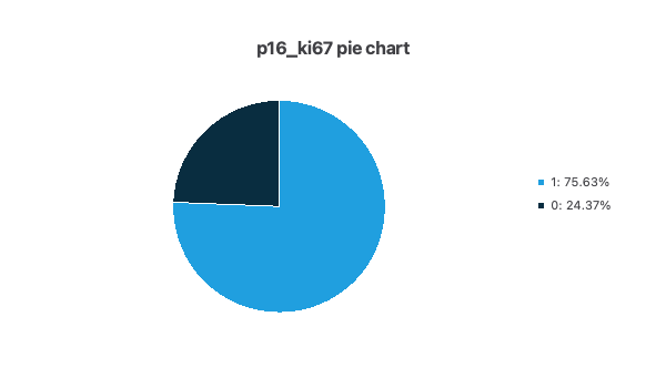
• The following pie chart shows the histogram for the variable P16/KI67. As you can see, there are many more positive than negative cases.
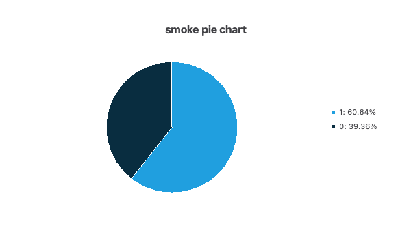
• The following pie chart shows the histogram for the variable SMOKE. As you can see, there are more smokers than non-smokers.
• The following chart shows the histogram for the variable PROGNOSIS. The maximum frequency is for cases with CIN II-III or CIN III, and the minimum is for patients with ADENOCARCINOMA or SQUAMOUS CARCINOMA.

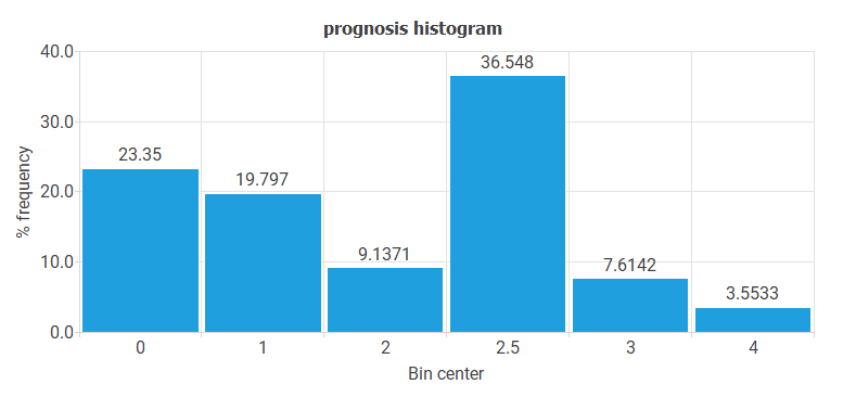
The most important conclusion from all these histograms is that there is little data on the most severe pathologies (ADENOCARCINOMA or SQUAMOUS CARCINOMA). These pathologies are precisely the ones we are most interested in predicting.

Correlations

It might be interesting to look for linear dependencies or correlations between the input and target variables.
Correlations near 1 mean that the prognosis has a strong linear dependence on an input. Conversely, correlations close to 0 indicate no linear relationship between that input and the prognosis.
Note that, in general, target variables depend on many inputs simultaneously, and their relationship is not linear.
The following chart shows the linear correlations between all inputs and the prognosis.

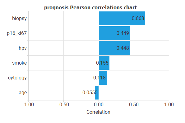
As you can see, the minimum correlations are for the variables AGE and CYTOLOGY, and the maximum correlations are for BIOPSY and P16/KI67.
These correlations can indicate the relative importance of each variable in the prognosis. However, we must be careful with these results since many variables are usually involved in cancer development.

4. Neural network

The neural network defines a function that represents the prognostic model.
The neural network employed here is based on the multilayer perceptron. This type of model is widely used due to its good approximation properties. The multilayer perceptron is extended with a scaling layer connected to the inputs and a de-scaling layer attached to the outputs. These two layers make the neural network always work with normalized values, thus producing better results. As well as the mentioned layers, there is one final bounding layer. Initially, the number of inputs to the neural network is six (AGE, CYTOLOGY, HPV, BIOPSY, P16/KI67, and SMOKE), and the number of outputs is one (PROGNOSIS).
The generalization study eliminates variables that do not improve the predictive capabilities of the neural network. The complexity of this neural network is two layers of perceptrons. The first layer, or hidden layer, has a sigmoidal activation function. The second layer, or output layer, has a linear activation function. Initially, the number of neurons in the hidden layer is ten, although the generalization study may reduce or increase that number until it finds the optimal complexity.
The following graph is a graphical representation of the neural network. As mentioned above, it contains a scaling layer in yellow, two perceptron layers in blue, a red unscaling layer, and a purple bounding layer.

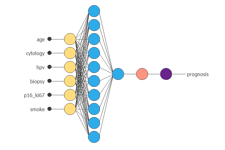
The figure above takes six input values (AGE, CYTOLOGY, HPV, BIOPSY, P16/KI67, and SMOKE) to produce one output value (PROGNOSIS).

5. Training strategy

The fourth step is to set the training strategy, which is composed of two terms:

• A loss index.
• An optimization algorithm.

Loss index

The loss index mainly measures the fit between the neural network and the data. It takes high values if the neural network does not fit the data well.
This application uses the normalized squared error as the target term. A normalization coefficient divides the sum of squared errors between the neural network outputs and their corresponding targets in the data set.
If the normalized squared error is 1, the neural network predicts the data ‘on the mean’, while 0 means a perfect data prediction. The loss index also measures the complexity of the neural network. For example, if the neural network undergoes oscillations, it takes high values.
We use the L2 as a regularization term. It is applied to control the neural network’s complexity by reducing the parameters’ value. The following table summarizes the objective and regularization terms used in the performance function.

The error and regularization terms in the table above are widely used in neural networks.

Optimization algorithm

The training (or learning) strategy is the procedure that performs the learning process. It is applied to the neural network to obtain the best possible representation.
We use the quasi-Newton method as the optimization algorithm. It is based on Newton’s method but does not require second derivative calculations. Instead, the quasi-Newton method approximates the second derivatives using information from the first derivatives.
The following table shows the operators, parameters, and stopping criteria of the quasi-Newton method used in this study.

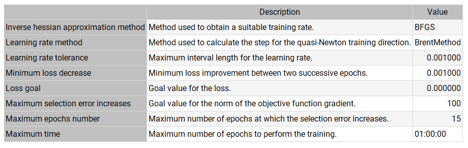
Note that the quasi-Newton method is one of the most widely used training strategies in neural networks.

6. Model selection

To know if the predictive capabilities of a neural network are reasonable, we use the selection samples from the data. The error of the neural network on this data indicates the capacity of the model to predict future cases not included in the set used for training.
The generalization study looks for the neural network with the optimal topology, testing several different models and selecting the one that produces the lowest selection error. In this sense, it trains several neural networks by eliminating input variables and measures the selection error.
The result is that the predictive capabilities improve by eliminating the variable SMOKE. However, by eliminating any other variable, the predictive capabilities worsen.
On the other hand, several neural networks with different complexities have been trained, also measuring the selection error. The result is an optimal complexity of two neurons in the hidden layer.
The following table shows the training results that produced the lowest selection error.

The final training error is small (0.444), showing that the neural network fits the data. The selection error is also small (0.477), indicating that the neural network has good predictive capabilities.
The training algorithm required 43 epochs, which required 0 s of computation.
The following figure shows the neural network resulting from the lowest generalization error. As we can see, the number of inputs is 5 (CYTOLOGY, HPV, BIOPSY, P16/KI67, and SMOKE), and the number of neurons in the hidden layer is 2. This is the optimal topology for this prognostic problem.

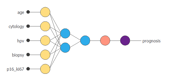
7. Testing analysis

The testing analysis compares the results predicted by the neural network and their respective values in an independent data set. The neural network can move to the production phase if the validation analysis is acceptable.
A standard method to validate the quality of a predictive model is to perform a linear regression analysis between the neural network outputs and the corresponding target values in the data set for an independent validation subset.
This analysis leads to the parameter R2, the correlation coefficient between outputs and targets. If we had a perfect fit (outputs equal to targets), the ordinate at the origin would be 0, the slope would be 1, and the correlation coefficient would be 1.
The following table shows the linear regression parameters for our case study.

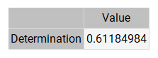
As we can see, the correlation coefficient (0.612) is close to 1. These three values indicate that the neural network predicts the validation data relatively well. However, these predictions are subject to improvement.
The following figure shows the linear regression between the predicted values and their corresponding actual values for the variable PROGNOSIS.

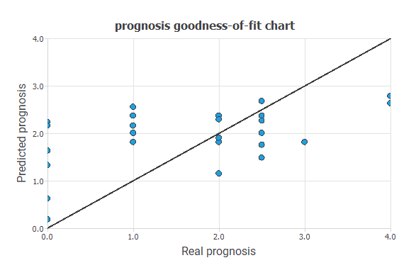
The black line indicates a perfect fit. As we can see, the trend is good, and the dispersion is not very high, although they are also susceptible to improvement.

Error statistics

Exploring the errors made by the neural network in each validation case is convenient. The absolute error is the difference between some target and its corresponding output. The relative error is the absolute error divided by the range of the variable. Finally, the percentage error is the relative error multiplied by 100.
The following table shows the basic error statistics for the validation cases. The mean error is 0.5, half a degree on the PROGNOSIS variable. This is a good indicator of the quality of the diagnoses.

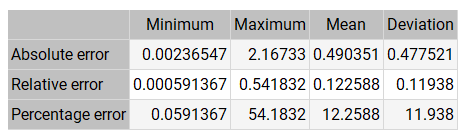
On the other hand, the table above shows some high errors. Therefore, we need to study whether these are isolated cases.

8. Model deployment

Once we have validated the predictive capabilities of the neural network, the cervical pathology unit can use it as a decision support system.
The following equation lists the mathematical expression represented by the neural network. It inputs the values of CYTOLOGY, HPV, BIOPSY, P16/KI67, and SMOKE to produce the output PROGNOSIS.

scaled_age = (age-39.73600006)/9.727999687;
scaled_cytology = (cytology-1.421880007)/1.543300033;
scaled_hpv = (hpv-2.333329916)/0.9072650075;
scaled_biopsy = (biopsy-1.636600018)/1.094120026;
scaled_p_one__six__ki_six__seven_ = p_one__six__ki_six__seven_*(1+1)/(1-(0))-0*(1+1)/(1-0)-1;
perceptron_layer_1_output_0 = tanh( 0.115422 + (scaled_age*-0.0455241) + (scaled_cytology*-0.285325) + (scaled_hpv*-0.0672079) + (scaled_biopsy*-0.427873) + (scaled_p_one__six__ki_six__seven_*0.364217) );
perceptron_layer_1_output_1 = tanh( -0.436525 + (scaled_age*-0.76002) + (scaled_cytology*-2.19671) + (scaled_hpv*1.51483) + (scaled_biopsy*-0.0450644) + (scaled_p_one__six__ki_six__seven_*2.33392) );
perceptron_layer_2_output_0 = ( 0.340502 + (perceptron_layer_1_output_0*-1.85234) + (perceptron_layer_1_output_1*0.595737) );
unscaling_layer_output_0=perceptron_layer_2_output_0*1.155930042+1.66497004;

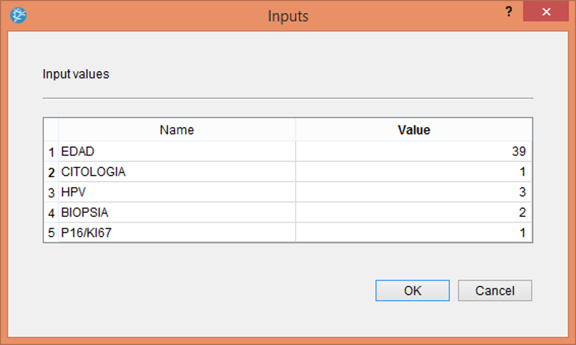
The information here is propagated forward through the scaling layer, the perceptron layers, and the de-scaling layer.
The following figure shows the use of the neural network for decision support within the Neural Designer software. This consists of the physician entering the values corresponding to the patient: age, cytological result, HPV type, cervical biopsy result, and positivity or not for p16.

Once we enter the previous values, the program produces a table with the prognosis calculated for that patient, as shown in the following table.

The patient would be 39, ASC-US cytology, HPV 16, CIN II biopsy, and P16/KI67 positive.
The PROGNOSIS estimated by the neural network for that patient would be 1.95, corresponding to a CIN II.

Conclusions

Concerning the results obtained, and always bearing in mind the limitations of a study of this nature, we draw the following conclusions:

• The demographic and epidemiological characteristics of the women participating in the cervical cancer screening program in the Palencia Health Area are similar to those identified in the national and regional context:
  • Women residing in Palencia (Spain)
  • 24 to 64 years of age
  • With sexual relations
  • With gynecological symptoms
• Applying an artificial neural network in the cervical pathology unit based on a population-based cervical cancer screening program, we can identify relevant variables for classifying the participating women already in the unit.
• In our study, the neural network model applied is the Multilayer Perceptron, as it is the one that best suits our prognostic needs. This type of neural network is widely used in the medical field.
• In the follow-up of low-grade intraepithelial lesions (L-SIL), the Neural Network created for our Cervical Pathology Unit is an effective predictor in selecting those that would evolve into high-grade lesions and prevent them from going unnoticed.
• When selecting only those patients with CIN II and studying their probability of developing cervical carcinoma, we found the failure due to the lack of existing data in the unit.
• The interaction of the risk factors evaluated makes the proposed neural network model efficient and helps us identify women at risk of cervical cancer. Furthermore, it helps us identify the women participating in the screening program in risk groups for developing cervical cancer.
• The machine learning model appears to facilitate the design of follow-up programs based on the risk profile of the participating women already classified and followed up in a cervical pathology unit.
• Concerning what we have observed in our study, we can affirm that, in general, artificial neural networks make it possible to propose on-demand a la carte clinical follow-ups according to relevant predictors, improving the quality of the research, minimizing clinical actions on the patients and optimizing the management of resources. We must continue implementing their information, increasing the data, and introducing and assessing more variables that may influence the final prognosis.
• Artificial Neural Networks are a powerful tool for analyzing the data set.

References

• Cervical cancer early detection program in Castilla y Leon data collected by the Cervical Pathology Unit in the health area of Palencia (Castilla y León).

Related posts