In this example, we build a machine learning model to predict employee churn and help companies reduce staff turnover.
Employee attrition is one of the biggest challenges for human resources.
It is costly, since keeping an employee is far less expensive than hiring and training a new one.
The goal is to predict who might leave, when they might leave, and why they might leave.
With accurate predictions, organizations can take action early, address the leading causes of turnover, and improve employee retention.
Contents
1. Application type
This is a classification project since the variable to be predicted is binary (attrition or not).
The goal here is to model the probability of attrition, conditioned on the employee features.
2. Data set
Data source
The data file employee_attrition.csv contains quantitative and qualitative information about a sample of employees at the company.
The data set contains about 1,500 employees (or instances).
For each, around 35 personal, professional, and socio-economic attributes (or variables) are selected.
Variables
More specifically, the variables of this example are the following.
Demographics
- Age
- Gender: Male, Female
- Marital status: Single, Divorced, Married
- Over 18: True or False
Job Information
- Department: Sales, Research & Development, Human Resources
- Job role: Sales Executive, Research Scientist, Laboratory Technician, Manufacturing Director, Healthcare Representative, Manager, Sales Representative, Research Director, Human Resources
- Job level: 1–5
- Job involvement: 1–4
- Years at company
- Years in current role
- Years since last promotion
- Years with current manager
Compensation
- Daily rate
- Hourly rate
- Monthly income
- Monthly rate
- Percent salary hike
- Stock option level: 0–3
Performance & Engagement
- Performance rating
- Job satisfaction: 1–4
- Environment satisfaction: 1–4
- Relationship satisfaction: 1–4
- Work-life balance: 1–4
- Training times last year
Career History
- Number of companies worked
- Total working years
- Business travel: Non-travel (0), Rarely (1), Frequently (2)
- Distance from home
Education
- Education: 1–5
- Education field: Life Sciences, Human Resources, Medical, Marketing, Technical Degree, Other
Administrative
- Employee count
- Employee number
- Standard hours
- Over time: True or False
Target Variable
Attrition: Loyal or Attrition
Variables distribution
Before starting the predictive analysis, it is important to know the distributions of the variables.
The following pie chart shows the ratio of negative and positive instances.
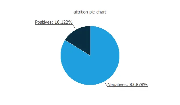
The chart above shows that the data is unbalanced, i.e., the number of negative instances (1233) is much larger than that of positive instances (237).
We use this information later to design the predictive model properly.
Input-target correlations
The input-target correlations analyze the dependencies between each input variable and the target.
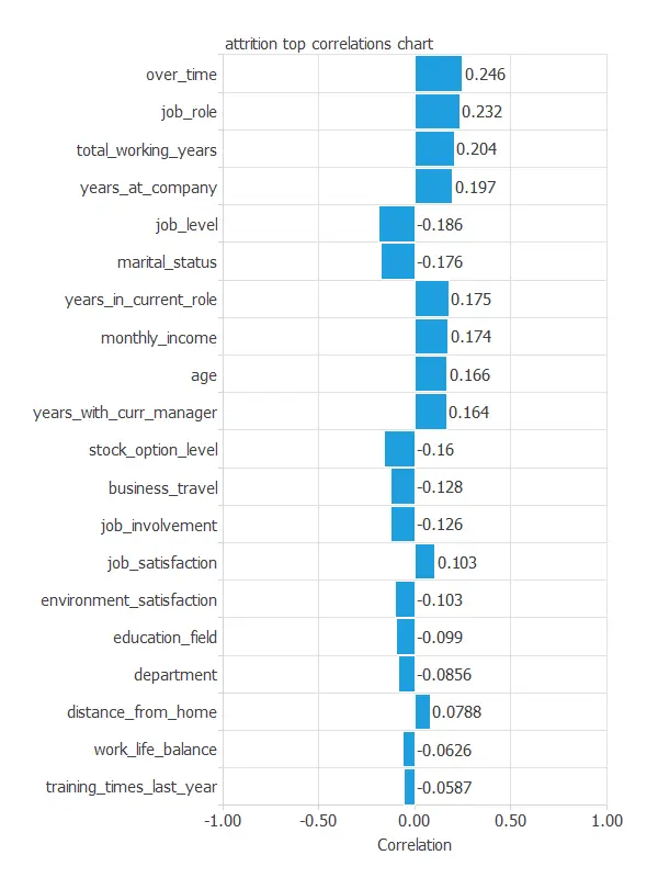
As we can see, the input variables that have more importance in the attrition are “over time” (0.246), “total working years” (0.223), and “years at company” (0.196).
3. Neural network
The neural network takes all the employees’ attributes and transforms them into a probability of attrition.
For that purpose, we use a neural network composed of a scaling layer with 48 neurons, a perceptron layer with 3 neurons, and a probabilistic layer with 1 neuron.
4. Training strategy
The next step is to select an appropriate training strategy that defines what the neural network will learn.
A general training strategy is composed of two concepts:
- A loss index.
- An optimization algorithm.
Loss index
As mentioned earlier, the dataset is unbalanced.
To address this, we use the weighted squared error as the error method.
This assigns a weight of 5.20 to positive instances and 1 to negative ones.
With this adjustment, the total weight of positives equals that of negatives.
Optimization algorithm
We use the quasi-Newton method as the optimization algorithm.
Now, the model is ready to be trained. The following chart shows how the training and selection errors decrease with the epochs of the optimization algorithm.
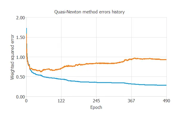
The final errors are 0.285 WSE for training and 0.931 WSE for validation.
5. Model selection
The objective of model selection is to find the network architecture with the best generalization properties, that is, the one that minimizes the error on the selected instances of the data set.
More specifically, we aim to develop a neural network with a selection error of less than 0.931 WSE, the current best value we have achieved.
Order selection algorithms train several network architectures with a different number of neurons and select the one with the smallest selection error.
The incremental order method starts with a small number of neurons and increases the complexity at each iteration. The following chart shows the training error (blue) and the selection error (orange) as a function of the number of neurons.
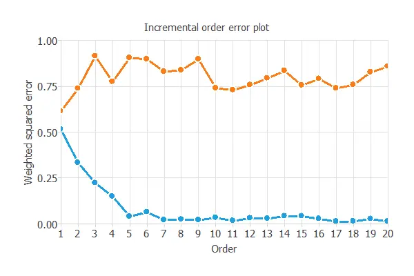
As we can see, the optimal number of neurons in the hidden layer is 1, resulting in an order selection error of 0.614 WSE, which is far better than the previous one.
6. Testing analysis
The testing analysis assesses the model’s quality to determine its readiness for use in the production phase, i.e., in a real-world situation.
The way to test the model is to compare the trained neural network’s outputs against the real targets for a data set that has been used neither for training nor selection, the testing subset.
For that purpose, we use some testing methods commonly used in binary classification problems.
ROC curve
The ROC curve measures the discrimination capacity of the classifier between positive and negative instances.
The ROC curve should pass through the upper left corner for a perfect classifier.
The following chart shows the ROC curve of our problem.
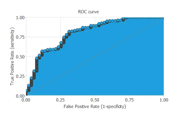
In this case, the area takes the value of 0.804, which confirms what we saw in the ROC chart, that the model predicts attrition with high accuracy.
Confusion matrix
For classification models with a binary target variable, constructing the confusion matrix is also a good task to test the model. Below, this table is displayed.
| Predicted positive | Predicted negative | |
|---|---|---|
| Real positive | 35 (11.9%) | 16 (5.44%) |
| Real negative | 47 (16%) | 196 (66.7%) |
Binary classification metrics
The following list depicts the binary classification tests. They are calculated from the values of the confusion matrix.
- Classification accuracy: 78.6% (ratio of correctly classified samples).
- Error rate: 21.4% (ratio of misclassified samples).
- Sensitivity: 68.6% (percentage of actual positives classified as positive).
- Specificity: 80.6% (percentage of actual negatives classified as negative).
In general, these binary classification tests show a good performance of the predictive model.
Nevertheless, it is essential to highlight that this model has greater specificity than sensitivity, showing that it works better when detecting negative instances accurately.
7. Model deployment
Once we know that the model can accurately predict employee attrition, it can be used to evaluate employee satisfaction with the company. This is called model deployment.
The model takes the form of a function that takes an employee’s inputs and provides the predicted output.
Using the predictive model, we can simulate different scenarios and find the most significant factors for the attrition of a given employee.
This information allows the company to act on those variables.
Conclusions
Predicting employee churn helps organizations reduce the high costs of staff turnover.
By analyzing key factors such as job satisfaction, years at the company, and compensation, machine learning models can identify employees at risk of leaving.
With this knowledge, HR teams can take proactive measures to improve retention and strengthen organizational stability.