The objective of this example is to predict the default risk of a bank’s customers using machine learning.
The primary outcome of this project is to reduce loan losses and achieve real-time scoring and limited monitoring.
This example focuses on a customer’s default payments at a bank.
From a risk management perspective, the result of the predictive model’s probability of default will be more valuable than simply classifying clients as credible or not credible.
The credit risk database used here concerns consumers’ default payments in Taiwan.
This example is solved with Neural Designer. You can use the free trial to follow it step by step.
Contents
1. Application type
The variable we are predicting is binary (default or not). Therefore, this is a classification project.
The goal here is to model the probability of default as a function of the customer features.
2. Data set
The data set consists of four concepts:
- Data source.
- Variables.
- Instances.
- Missing values.
Data source
The data file credit_risk.csv contains the information used to create the model. It consists of 30,000 rows and 25 columns. The columns represent the variables, while the rows represent the instances.
Variables
This data set uses the following 23 variables:
Demographics
- Sex: Gender (1 = male, 2 = female).
- Education level: Highest education attained (1 = graduate school, 2 = university, 3 = high school, 4 = other).
- Marital status: 1 = married, 2 = single, 3 = other.
- Age: Age of the client (in years).
Credit Information
Limit balance: Amount of credit granted in NT dollars (includes personal and family/supplementary credit).
Repayment History
Repayment status (lag 1–6): Repayment status for the last 6 months (-1 = paid duly, 1 = one month delay, …, 9 = nine months delay or more).
Billing History
Bill statement amount (lag 1–6): Bill amount for each of the past 6 months (NT dollars).
Payment History
Payment amount (lag 1–6): Amount paid for each of the past 6 months (NT dollars).
Target Variable
Default: Indicates loan default (failure to repay).
Instances
Finally, the use of all instances is selected.
Each customer represents an instance that contains the input and target variables.
Neural Designer automatically splits the data into 60% training, 20% validation, and 20% testing.
In this case, that means 18,000 samples for training, 6,000 for validation, and 6,000 for testing.
Variables distribution
We can also calculate the data distributions for each variable.
The following figure depicts the number of customers who repay the loan and those who do not.
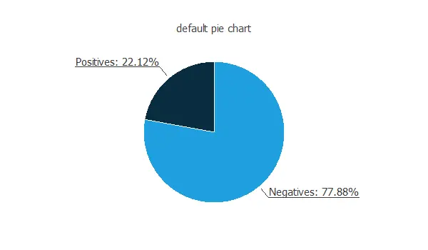
The data is unbalanced, as we can observe; this information will be used to configure the neural network later.
Input-target correlations
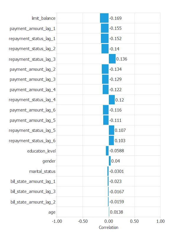
The following figure depicts the input-target correlations of all the inputs with the target.
This helps us understand the impact of various inputs on the default.
3. Neural network
The second step is to select a neural network that represents the classification function.
For classification problems, it is composed of:
- A scaling layer.
- A hidden dense layer.
- An output dense layer.
Scaling layer
The mean and standard deviation scaling method is set for the scaling layer.
Dense layers
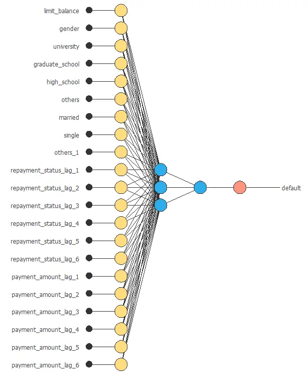
We set up two dense layers: one hidden layer with 3 neurons as a first guess and one output layer with 1 neuron, both layers having the logistic activation function.
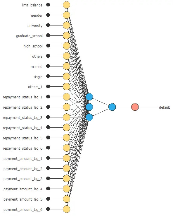
Neural network graph
The following figure shows the neural network used in this example.
4. Training strategy
The fourth step is to configure the training strategy, which is composed of two concepts:
- A loss index.
- An optimization algorithm.
Loss index
The error term is the weighted squared error. It weights the squared error of negative and positive values. If the weighted squared error has a value of unity, then the neural network predicts the data ‘in the mean’, while a value of zero means a perfect prediction of the data.
In this case, the neural parameters norm weight term is 0.01. This parameter makes the model stable, avoiding oscillations.
Optimization algorithm
The optimization algorithm is applied to the neural network to achieve optimal performance.
We chose the quasi-Newton method and left the default parameters.
The following chart illustrates how training and selection errors decrease over the course of training epochs.
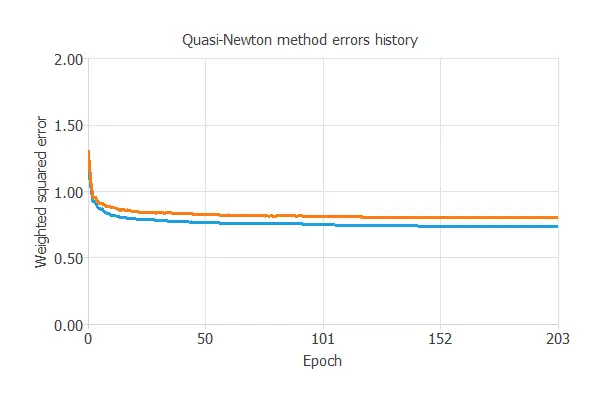
The final results are training error = 0.755 WSE and selection error = 0.802 WSE, respectively.
5. Model selection
A model selection aims to find the network architecture with the best generalization properties, i.e., the one that minimizes the error on the selected instances of the data set.
More specifically, we aim to develop a neural network with a selection error of less than 0.802 WSE, the current best value we have achieved.
Neuron selection
Order selection algorithms train several network architectures with different numbers of neurons and select the one with the smallest selection error.
The incremental order method starts with a few neurons and increases the complexity at each iteration.
The following chart shows the training error (blue) and the selection error (orange) as a function of the number of neurons.
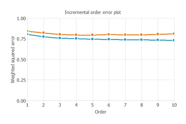
The final selection error achieved is 0.801 for an optimal number of neurons of 3.
The graph above represents the architecture of the final neural network.
6. Testing analysis
The next step is to evaluate the trained neural network’s performance through exhaustive testing analysis.
The standard way to do this is to compare the neural network’s outputs against previously unseen data, the training instances.
ROC curve
A common way to measure generalization is with the ROC curve, which shows how well the classifier separates the classes.
Its primary metric is the area under the curve (AUC), where values closer to 1 indicate better performance.
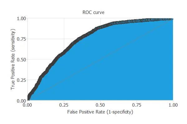
In this case, the AUC takes a high value: AUC = 0.772.
Confusion matrix
This matrix contains the variable class’s true positives, false positives, false negatives, and true negatives.
The following table contains the elements of the confusion matrix.
| Predicted positive | Predicted negative | |
|---|---|---|
| Real positive | 745 (12.4%) | 535 (8.92%) |
| Real negative | 893 (14.9%) | 3287 (63.8%) |
Binary classification tests
The binary classification tests are parameters for measuring the performance of a classification problem with two classes:
- Accuracy: 76.2% (ratio of correctly classified samples).
- Error: 23.8% (ratio of misclassified samples).
- Sensitivity: 58.2% (percentage of actual positives classified as positive).
- Specificity: 81.0% (percentage of actual negatives classified as negative).
The classification accuracy is high (76.2%), indicating that the prediction is effective in many cases.
Cumulative gain
Cumulative gain analysis shows how much better a predictive model is compared to random guessing.
It has three lines: the baseline (no model), the positive gain (percentage of positives found vs. population), and the negative gain (percentage of negatives found vs. population).
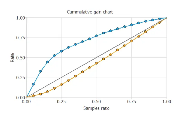
In this case, the model shows that by analyzing 50% of clients most likely to default, we can identify over 75% of actual defaulters.
7. Model deployment
Once the neural network’s generalization performance has been tested, it can be saved for future use in the so-called model deployment mode.
References
- UCI Machine Learning Repository. Default of credit card clients data set.
- Yeh, I. C., & Lien, C. H. (2009). The comparisons of data mining techniques for the predictive accuracy of probability of default of credit card clients. Expert Systems with Applications, 36(2), 2473-2480.