1. Application type
This is a classification project since the variable to be predicted is binary (fraudulent or legal).
The goal is to model the probability that a banknote is fraudulent as its features function.
2. Data set
The data file banknote_authentication.csv is the source of information for the classification problem. The number of instances (rows) in the data set is 1372, and the number of variables (columns) is 5.
In that way, this problem has the following variables:
- variance_of_wavelet_transformed, used as input.
- skewness_of_wavelet_transformed, used as input.
- curtosis_of_wavelet_transformed, used as input.
- entropy_of_image, used as input.
- counterfeit, used as the target. It can only have two values: 0 (non-counterfeit) or 1 (counterfeit).
The instances are divided into training, selection, and testing subsets. There are 824 instances for training (60%), 274 cases for selection (20%), and 274 cases for testing (20%).
We can calculate the data distributions and plot a pie chart with the percentage of instances for each class.
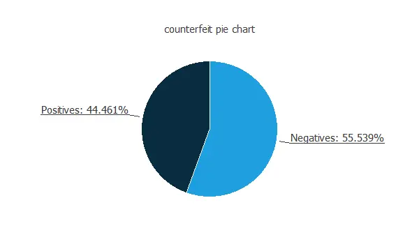
We can see that the numbers of authentic and forged banknotes are similar.
Next, we plot a scatter chart with the counterfeit and the wavelet transformed variance data.
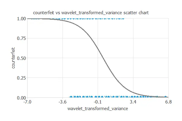
In general, the more wavelet transformed variance, the less counterfeit probability.
The inputs-targets correlations might indicate which factors better discriminate between authentic and false banknotes.
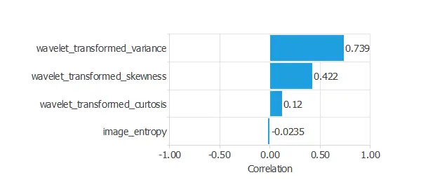
The above chart shows that the wavelet transformed variance might be the most influential variable for this application.
3. Neural network
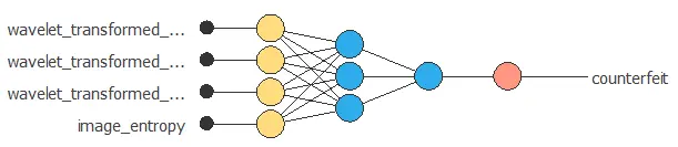
The second step is configuring a neural network to represent the classification function.
The following picture shows the neural network that defines the model.
4. Training strategy
The fourth step is to set the training strategy, which is composed of:
- Loss index.
- Optimization algorithm.
The loss index that we use is the weighted squared error with L2 regularization.
We can state the learning problem as finding a neural network that minimizes the loss index. That is, we want a neural network that fits the data set (error term), and that does not oscillate (regularization term).
We use here the quasi-Newton method as the optimization algorithm. The default training parameters, stopping criteria, and training history settings are left.
The following figure shows the loss history with the quasi-Netwon method. As we can see, the loss decreases until it reaches a stationary value. This is a sign of convergence.
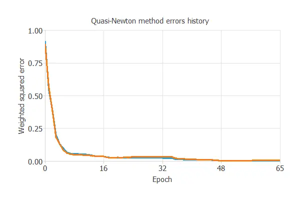
The final training and selection errors are almost zero, which means the neural network fits the data well.
More specifically, training error = 0.014 WSE and selection error = 0.011 WSE.
5. Model selection
The objective of model selection is to improve the neural network’s generalization capabilities or, in other words, to reduce the selection error.
Since the selection error we have achieved so far is minimal (0.011 WSE), there is no need to apply an order or input selection.
6. Testing analysis
The testing analysis aims to validate the generalization performance of the trained neural network.
A good measure for the precision of a binary classification model is the ROC curve.
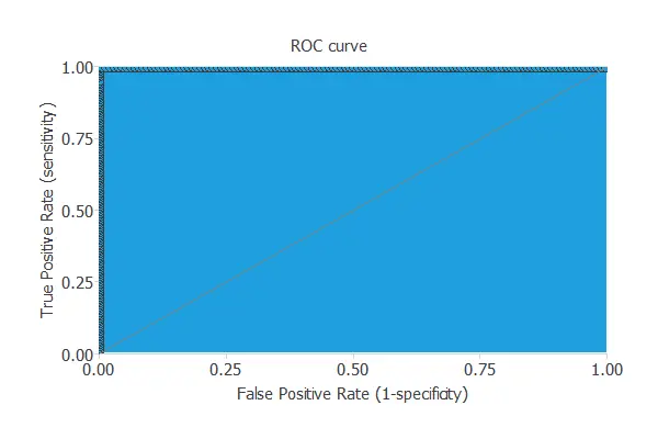
The area under the model’s curve is AUC = 1, which means that the classifier predicts all the testing instances well.
In the confusion matrix, the rows represent the target classes, and the columns the output classes for the testing target data set. The diagonal cells in each table show the number of correctly classified cases, and the off-diagonal cells show the misclassified instances. The following table contains the elements of the confusion matrix.
| Predicted positive | Predicted negative | |
|---|---|---|
| Real positive | 103 | 0 |
| Real negative | 0 | 171 |
The number of correctly classified instances is 274, and the number of misclassified cases is 0. As there are no misclassified patterns, the model predicts this testing data well.
7. Model deployment
In the model deployment phase, the neural network predicts outputs for inputs it has never seen.
For that, we can use Response Optimization. The objective of the response optimization algorithm is to exploit the mathematical model to look for optimal operating conditions. Indeed, the predictive model allows us to simulate different operating scenarios and adjust the control variables to improve efficiency.
An example is maximizing wavelet variance while maintaining the result equal to 1.
The following table resumes the conditions for this problem.
| Variable name | Condition | |
|---|---|---|
| Variance of wavelet | Maximize | |
| Skewness of wavelet | None | |
| Curtosis of wavelet | None | |
| Entropy of image | None | |
| Counterfeit | Greater than | 0.5 |
The following list shows the optimum values for previous conditions.
- variance_of_wavelet_transformed: 6.62294.
- skewness_of_wavelet_transformed: -10.5761.
- curtosis_of_wavelet_transformed: -2.55656.
- entropy_of_image: 1.39497.
- counterfeit: 0.98 (98% of been fraudulent).
We can embed the neural network’s mathematical expression in the banknote authentication system. This expression is written below.
scaled_wavelet_transformed_variance = (wavelet_transformed_variance-0.433735)/2.84276;
scaled_wavelet_transformed_skewness = (wavelet_transformed_skewness-1.92235)/5.86905;
scaled_wavelet_transformed_curtosis = (wavelet_transformed_curtosis-1.39763)/4.31003;
scaled_image_entropy = (image_entropy+1.19166)/2.10101;
y_1_1 = Logistic (-2.95122+ (scaled_wavelet_transformed_variance*-3.20568)+ (scaled_wavelet_transformed_skewness*-4.57895)
+ (scaled_wavelet_transformed_curtosis*-5.83131)+ (scaled_image_entropy*0.125717));
y_1_2 = Logistic (3.23366+ (scaled_wavelet_transformed_variance*3.5863)+ (scaled_wavelet_transformed_skewness*2.36407)
+ (scaled_wavelet_transformed_curtosis*1.0865)+ (scaled_image_entropy*-1.0501));
non_probabilistic_counterfeit = Logistic (3.48838+ (y_1_1*9.72432)+ (y_1_2*-8.93277));
(counterfeit) = Probability(non_probabilistic_counterfeit);
Logistic(x){
return 1/(1+exp(-x))
}
Probability(x){
if x < 0
return 0
else if x > 1
return 1
else
return x
}
8. Conclusions
References
- Banknote authentication data set, UCI Machine Learning Repository.