This example aims to target customers and predict whether bank clients will subscribe to a long-term deposit using machine learning.
Customer targeting involves identifying individuals who are more likely to be interested in a specific product or service.
The data set used here is related to the direct marketing campaigns of a Portuguese bank institution.
This example is solved with Neural Designer. To follow it step by step, you can use the free trial.
Contents
1. Application type
The variable to be predicted is binary (i.e., whether to buy or not). Thus, this is a classification project.
The goal here is to model the probability of buying as a function of the customer features.
2. Data set
In general, a data set contains the following concepts:
- Data source.
- Variables.
- Instances.
- Missing values.
The data file bank_marketing.csv contains the information used to create the model. It consists of 1522 rows and 19 columns. Each row represents a different customer, while each column represents a distinct feature for each customer.
The variables are:
Demographics
- Age: Client’s age.
- Marital status: Married, single, or divorced.
- Education: Level of education (primary, secondary, tertiary).
Financial Information
- Balance: Client’s account balance.
- Default: 1 if the client has a credit in default, 0 otherwise.
- Housing loan: 1 if the client has a housing loan, 0 otherwise.
- Personal loan: 1 if the client has a personal loan, 0 otherwise.
Campaign Information
- Contact type: Communication method (cellular or telephone).
- Last contact day: Day of the month the client was last contacted.
- Last contact month: Month of the year the client was last contacted.
- Campaign: Number of contacts during this campaign for the client.
- Pdays: Days since the client was last contacted from a previous campaign.
- Previous contacts: Number of contacts before this campaign.
- Previous outcome: Result of the previous marketing campaign.
Target Variable
Conversion: 1 if the client subscribed to a term deposit, 0 otherwise.
Instances
There are 1,522 instances in the dataset. 60% are used for training, 20% for selection, and 20% for testing.
Distributions
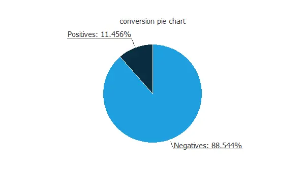 As expected, the number of calls without conversion is much greater than the number of calls with conversion.
Input-target correlations
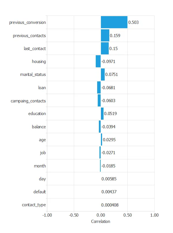
We can also calculate the input-target correlations between the conversion rate and all the customer features to see which variables might influence the buying process.
3. Neural network
The second step is to configure the neural network parameters. For classification problems, it is composed of:
- Scaling layer.
- Perceptron layers.
- Probabilistic layer.
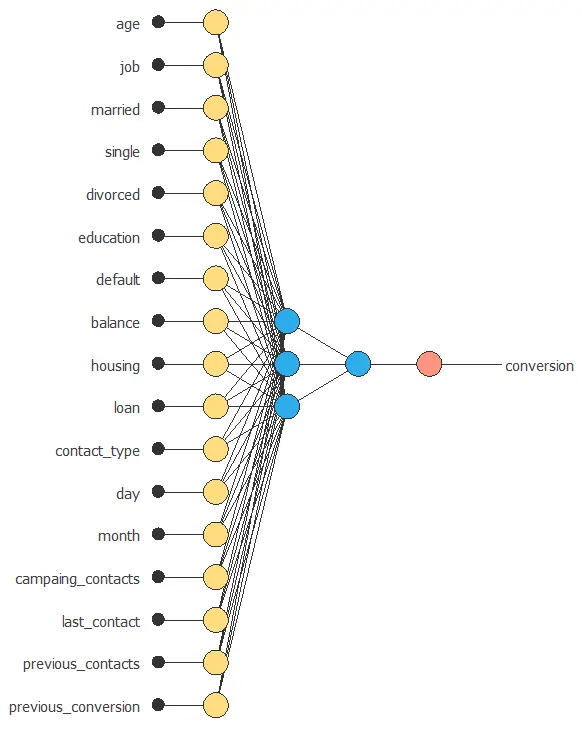
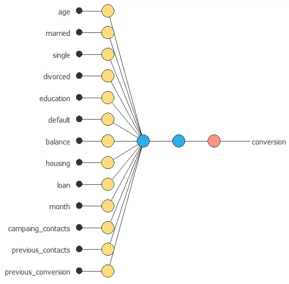
Neural network graph
The following figure is a graphical representation of the neural network used for this problem.
4. Training strategy
The fourth step is to configure the training strategy, which is composed of two concepts:
- A loss index.
- An optimization algorithm.
Loss index
The loss index chosen is the weighted squared error with L2 regularization.
Optimization algorithm
The optimization algorithm is applied to the neural network to get the minimum loss.
The chosen algorithm here is the quasi-Newton method. We leave the default training parameters, stopping criteria, and training history settings.
Training
The following chart illustrates how the training and selection errors decrease with the number of epochs during the training process.
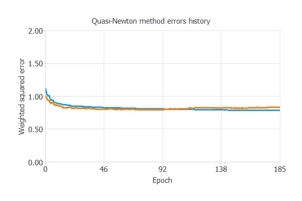
The final values are training error = 0.821 WSE and selection error = 0.889 WSE, respectively.
5. Model selection
The objective of model selection is to find a network architecture with the best generalization properties, that is, one that minimizes the error on the selected instances of the data set.
More specifically, we aim to find a neural network with a selection error of less than 0.889 WSE, which is the current best value we have achieved.
Order selection algorithms train several network architectures with different numbers of neurons and select the one with the smallest selection error.
The incremental order method starts with a small number of neurons and increases the complexity at each iteration. The following chart shows the training error (blue) and the selection error (orange) as a function of the number of neurons.
6. Testing analysis
The objective of the testing analysis is to evaluate the generalization performance of the neural network.
The standard way to do this is to compare the neural network outputs against data that it has never seen before, the testing instances.
ROC curve
A commonly used method to test a neural network is the ROC curve.
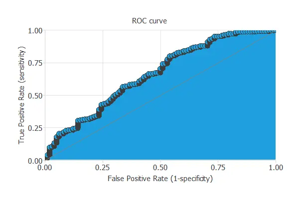
One of the parameters obtained from this chart is the area under the curve (AUC). The closer to 1 is the area under the curve, the better is the classifier. In this case, the area under the curve takes a high value: AUC = 0.80.
Binary classification metrics
The binary classification tests provide us with helpful information for testing the performance of a binary classification problem:
- Classification accuracy: 79.4% (ratio of correctly classified samples).
- Error rate: 20.6% (ratio of misclassified samples).
- Sensitivity: 80.4% (percentage of actual positives classified as positive).
- Specificity: 79.3% (percentage of actual negatives classified as negative).
The classification accuracy achieves a high value, indicating that the prediction is suitable for many cases.
Cumulative gain
The second is another visual aid that shows the advantage of using a predictive model against randomness.
The following picture depicts the cumulative gain for the current example.
As we can see, this chart shows that by calling only half of the clients, we can achieve more than 80% of the positive responses.
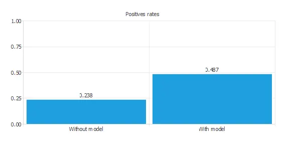
Positive rates
The conversion rates for this problem are depicted in the following chart.
7. Model deployment
In the model deployment phase, the neural network can be used for different techniques.
We can predict which clients have a higher probability of buying the product by calculating the neural network outputs.
We need to know the input variables for each new client.
References:
- UCI Machine Learning Repository. Bank marketing data set.