2. Data set
The data set contains three concepts:
- Data source.
- Variables.
- Instances.
The data file combined_cycle_power_plant.csv contains 9568 samples with five variables collected from a combined cycle power plant over six years when the power plant was set to work with a full load. The measurements were taken every second.
The variables, or features, are the following:
- temperature, in degrees Celsius.
- exhaust_vacuum, in cm Hg.
- ambient_pressure, in millibar.
- relative_humidity, in percentage.
- energy, in MW, net hourly electrical energy output.
The instances are divided into training, selection, and testing subsets. They represent 60%, 20%, and 20% of the original instances, respectively, and are randomly split.
Calculating the data distributions helps us check for the available information’s correctness and detect anomalies. The following chart shows the histogram for the variable energy_output.
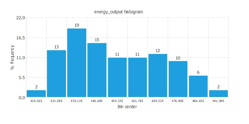
As we can see, there are more scenarios where the energy produced is small than where it is significant.
It is also interesting to look for dependencies between a single input and single target variables. To do that, we can plot an inputs-targets correlations chart.
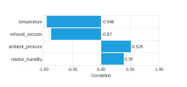
The temperature yields the highest correlation (generally, the higher the temperature, the less energy production).
Next, we plot a scatter chart for the energy output and the exhaust vacuum.
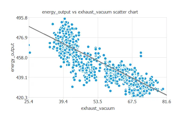
As we can see, the energy output is highly correlated with the exhaust vacuum. In general, the more exhaust vacuum, the less energy production.
3. Neural network
The second step is building a neural network representing the approximation function. Approximation models usually contain the following layers:
- Scaling layer.
- Perceptron layers.
- Unscaling layer.
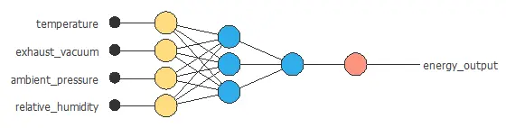
The neural network has four inputs (temperature, exhaust vacuum, ambient pressure, and relative humidity) and one output (energy output).
The scaling layer contains the statistics of the inputs. We use the mean and standard deviation scaling method as all inputs have normal distributions.
We use 2 perceptron layers here:
- The first perceptron layer has 4 inputs, 3 neurons, and a hyperbolic tangent activation function.
- The second perceptron layer has 3 inputs, 1 neuron, and a linear activation function.
The unscaling layer contains the statistics of the outputs. As the output has a normal distribution, we use the mean and standard deviation unscaling method.
The next graph represents the neural network for this example.
4. Training strategy
The fourth step is to select an appropriate training strategy. It is composed of two things:
- A loss index.
- An optimization algorithm.
Loss index
The loss index defines what the neural network will learn. It is composed of an error term and a regularization term.
The error term chosen is the normalized squared error. A normalization coefficient divides the squared error between the neural network outputs and the data set’s targets. If the normalized squared error has a value of 1, then the neural network predicts the data ‘in the mean’, while a zero value means a perfect data prediction. This error term does not have any parameters to set.
The regularization term is the L2 regularization. It is applied to control the neural network’s complexity by reducing the parameters’ value. We use a weak weight for this regularization term.
Optimization algorithm
The optimization algorithm is in charge of searching for the neural network parameters that minimize the loss index. Here, we chose the quasi-Newton method as the optimization algorithm.
Training process
The following chart shows how the training (blue) and selection (orange) errors decrease with the epochs during the training process.
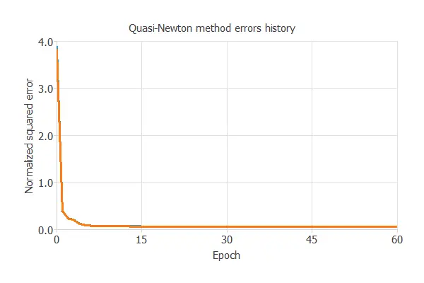
The final values are training error = 0.057 NSE and selection error = 0.067 NSE, respectively.
6. Testing analysis
The purpose of the testing analysis is to validate the generalization capabilities of the neural network. We use the testing instances in the data set, which have never been used before.
A standard testing method in approximation applications is to perform a linear regression analysis between the predicted and the real energy output values.
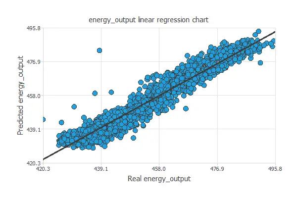
For a perfect fit, the correlation coefficient R2 would be 1. As we have R2 = 0.968, the neural network is predicting very well the testing data.
7. Model deployment
In the model deployment phase, the neural network predicts outputs for inputs it has never seen.
Neural network outputs
We can calculate the neural network outputs for a given set of inputs:
- temperature: 19 degrees Celsius.
- exhaust_vacuum: 54 cm Hg.
- ambient_pressure: 1013 millibar.
- relative_humidity: 73 %.
The predicted output for these input values is the following:
- energy_output: 452 MW.
Response optimization
The objective of the Response Optimization algorithm is to exploit the mathematical model to look for optimal operating conditions. Indeed, the predictive model allows us to simulate different operating scenarios and adjust the control variables to improve efficiency.
An example is minimizing exhaust vacuum while maintaining energy over the desired value.
The next table resumes the conditions for this problem.
| Variable name | Condition | |
|---|---|---|
| Temperature | None | |
| Exhaust vacuum | Minimize | |
| Ambient pressure | None | |
| Relative humidity | None | |
| Energy | Greater than or equal to | 450 |
The next list shows the optimum values for previous conditions.
- temperature: 19.3846 Celsius degrees.
- exhaust_vacuum: 25.432 cm Hg.
- ambient_pressure: 1021.4 millibar.
- relative_humidity: 60.8 %.
- energy: 462.086 MW.
Directional outputs
Directional outputs plot the neural network outputs through some reference points.
The next list shows the reference points for the plots.
- temperature: 19 Celsius degrees.
- exhaust_vacuum: 54 cm Hg.
- ambient_pressure: 1013 millibar.
- relative_humidity: 73 %.
Next, we define a reference point and see how the energy production varies with the exhaust vacuum around that point.
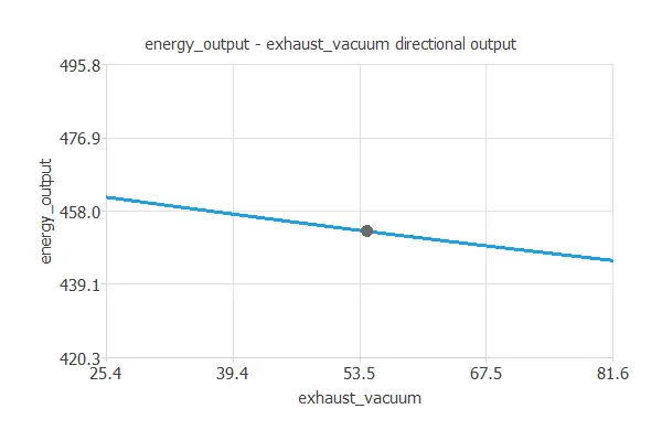
As we can see, reducing the exhaust vacuum increases energy output.
Mathematical expression
The mathematical expression represented by the predictive model is listed next:
scaled_temperature = (temperature-19.6512)/7.45247;
scaled_exhaust_vacuum = 2*(exhaust_vacuum-25.36)/(81.56-25.36)-1;
scaled_ambient_pressure = (ambient_pressure-1013.26)/5.93878;
scaled_relative_humidity = (relative_humidity-73.309)/14.6003;
y_1_1 = tanh(-0.158471 + (scaled_temperature*0.200864) + (scaled_exhaust_vacuum*0.73313)
                       + (scaled_ambient_pressure*-0.19189) + (scaled_relative_humidity*0.0133642));
y_1_2 = tanh(-0.290828 + (scaled_temperature*-0.020375) + (scaled_exhaust_vacuum*-0.263848)
                       + (scaled_ambient_pressure*-0.227397)+ (scaled_relative_humidity*0.337468));
y_1_3 = tanh(0.574054 + (scaled_temperature*0.572764) + (scaled_exhaust_vacuum*-0.0264721)
                      + (scaled_ambient_pressure*0.109944)+ (scaled_relative_humidity*0.00934301));
scaled_energy_output =  (0.162012+ (y_1_1*-0.382654) + (y_1_2*-0.126065) + (y_1_3*-0.748958));
energy_output = (0.5*(scaled_energy_output+1.0)*(495.76-420.26)+420.26);
8. Tutorial video
You can watch the step-by-step tutorial video below to help you complete this Machine Learning example
for free using the easy-to-use machine learning software Neural Designer.
References
- Pinar Tufekci, Prediction of full load electrical power output of a baseload operated combined cycle power plant using machine learning methods, International Journal of Electrical Power & Energy Systems, Volume 60, September 2014, Pages 126-140, ISSN 0142-0615.
- Heysem Kaya, Pinar Tufekci, Fikret S. Gurgen: Local and Global Learning Methods for Predicting Power of a Combined Gas & Steam Turbine, Proceedings of the International Conference on Emerging Trends in Computer and Electronics Engineering ICETCEE 2012, pp. 13-18 (Mar. 2012, Dubai).