Learning

Predict the generation of a solar plant using machine learning

Forecast three-hour solar generation from weather and solar position

This example builds a compact nonlinear surrogate for a Berkeley solar installation. Nine routinely available weather and timing variables are converted into an estimate of the energy generated during each three-hour period.

2,920three-hour records
9operational inputs
0.895testing R²
2,019testing MAE

Short-horizon generation estimates can support production planning, deviation analysis and expected-versus-actual monitoring. The model is deliberately lightweight, but professional use still requires timestamped forecasting, plant availability signals, unit calibration and validation on future operating periods.

1. Industrial challenge

This is an approximation problem: the network maps a three-hour operating context to the generation reported by the data source.

Plan expected productionTurn weather forecasts into a short-horizon generation estimate for plant and portfolio planning.
Detect underperformanceCompare measured production with a weather-adjusted expectation to prioritize inspection and cleaning work.
Evaluate scenariosQuantify how changing cloud cover, humidity or distance from solar noon affects the predicted operating point.

Potential users include solar plant managers, operations and maintenance teams, performance engineers, energy forecasters, portfolio operators and industrial analytics teams.

Plant operationsO&MPerformance engineeringEnergy forecastingPortfolio operations
Scope of this example. This is a data-driven surrogate for one historical installation. It estimates the dataset target; it is not a physical photovoltaic model, certified meter, dispatch instruction or revenue-settlement calculation.

2. Data set

The updated solar_power_generation.csv contains 2,920 records, nine inputs and one target. Each row represents a three-hour period. All input combinations are unique; one average_wind_speed value is missing and is imputed with the training statistic configured in the Neural Designer project.

VariableOperational meaningSource scale / range
distance_to_solar_noonAbsolute angular distance from solar noon0.0504 to 1.1414 rad
temperatureAmbient temperature42 to 78 °F
wind_directionCoded wind-direction sector1 to 36; approximately ten-degree sectors
wind_speedObserved wind speed1.1 to 26.6 mph
sky_coverCloud-cover category0 clear to 4 overcast
visibilityReported visibility0 to 10 mi
humidityRelative humidity14% to 100%
average_wind_speedAverage wind speed over the period0 to 40 mph
average_pressureAverage atmospheric pressure over the period29.48 to 30.53 inHg
power_generatedGeneration reported for the three-hour periodTarget; 0 to 36,580 dataset units
Unit discipline. The weather fields retain the source data scale. Before integrating a live data feed, document every physical unit and conversion explicitly. The target is presented as dataset generation units because the public source does not provide enough plant-meter metadata for a defensible engineering conversion.
Distribution of three-hour solar generation values
Zero-heavy target. About 45.2% of records report zero generation, and 62.7% fall in the first histogram interval.
Pearson correlations between solar generation and the nine inputs
Timing dominates. Distance from solar noon has the strongest inverse association in the regenerated Neural Designer report; humidity is also negatively associated with generation.
Solar generation against distance from solar noon with the fitted directional relationship

The scatter plot captures the expected decline away from solar noon, but also exposes a deployment issue: the unconstrained neural response can become negative and non-monotonic at the edge of the represented range. This is addressed explicitly in the deployment controls below.

The configured random split contains 1,752 training, 584 selection and 584 testing records.

3. Neural network

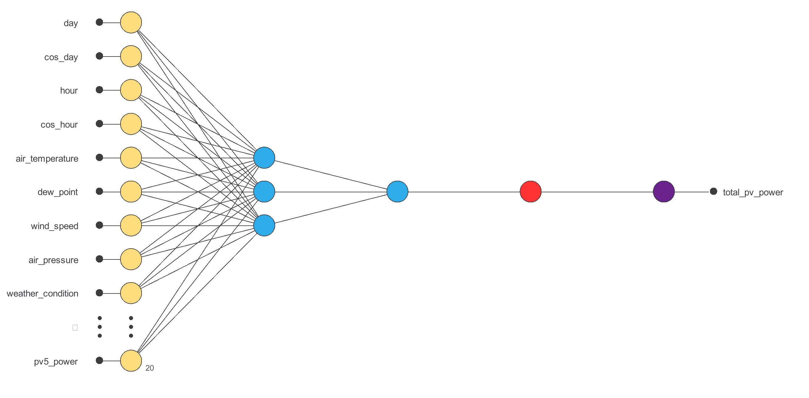
The baseline model standardizes the nine inputs, uses three tanh neurons in one hidden layer, and returns one continuous output through an identity activation and output unscaling.

Initial 9-3-1 solar generation neural network

This compact 9–3–1 architecture provides the starting point for training before the hidden-layer width is selected from held-out data.

4. Training strategy

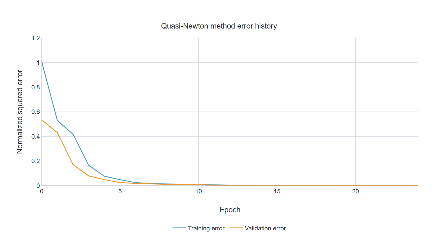
The network minimizes normalized squared error with the quasi-Newton method. Over 104 epochs, the training error falls from 1.0056 to 0.1477 and the selection error from 0.3451 to 0.0381.

Quasi-Newton training and selection error history for solar generation

The declining curves show stable convergence for the configured random split. They do not, by themselves, demonstrate performance on a future season or a different photovoltaic installation.

5. Model selection

The growing-neurons task evaluates hidden layers from one to ten neurons. The minimum selection error occurs with nine hidden neurons, reducing the selected training and selection errors to 0.1269 and 0.0323.

Training and selection errors for one to ten hidden neurons
The selection error reaches its minimum at nine neurons.
Final 9-9-1 solar generation neural network
The final 9–9–1 architecture matches the exported Python model used below.

6. Testing analysis

The final exported network is evaluated on the 584 testing records that were not used to fit its parameters or choose the hidden-layer size.

0.895coefficient of determination
2,019mean absolute error
3,225root mean squared error
-38.9mean prediction bias
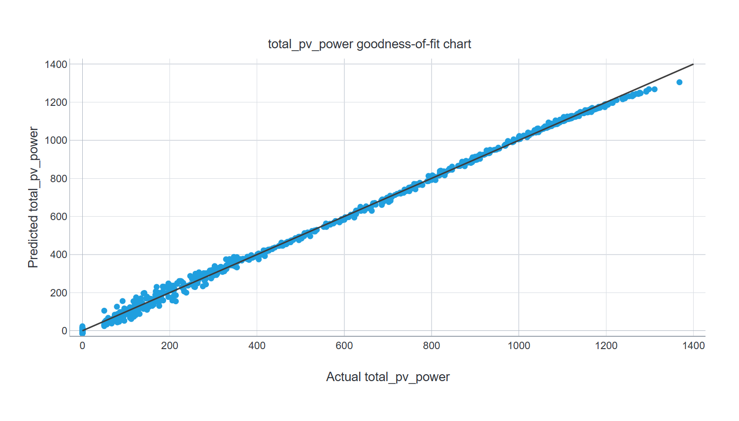
Goodness-of-fit chart for observed and predicted three-hour solar generation

The model explains approximately 89.5% of testing variance, but the chart shows compression at high generation: the network tends to underpredict some of the strongest production periods. The 95th percentile absolute error is about 7,042 dataset units, which is operationally more informative than R² alone when defining alert thresholds.

Physical output check. Raw testing predictions range from approximately -5,216 to 31,498 while generation cannot be negative. A production implementation should use a non-negative model/bounding layer or documented post-processing and should monitor how often that safeguard activates.

7. Model deployment

A professional workflow combines forecast or SCADA inputs with schema, unit and range checks; applies the trained surrogate; enforces physical operating rules; and records the forecast, model version and later measured production for monitoring.

Weather forecast and plant context
Schema, unit and range validation
Solar-generation surrogate
Physical bounds and operating decision

Representative near-noon operating case

This observed row from the dataset matches the reference point used in the regenerated directional-output analysis. It provides reproducible values for testing the downloaded Python model or the browser calculator.

InputValue
Distance to solar noon0.16623 rad
Temperature62 °F
Wind direction code29
Wind speed14.9 mph
Sky cover1 — low cloud
Visibility10 mi
Relative humidity68%
Average wind speed14 mph
Average pressure29.77 inHg
ResultDataset units / 3 h
Observed generation24,553
Model prediction22,254.3
Prediction error-2,298.7 (-9.4%)

Interpretation: the model estimates 22,254.3 units, around 9.4% below the observed value. For a plant manager, this single estimate is not an alarm threshold; it is a reproducible baseline that can be combined with an error band and later compared with the meter reading to identify sustained underperformance.

Distance-to-solar-noon scenario analysis

Holding the remaining reference inputs fixed, the directional-output task shows the estimated production profile as the operating period moves away from solar noon.

Directional output of solar generation across distance from solar noon

The central decline is operationally intuitive; the negative and upward-turning tail is not. Treat it as evidence that the unconstrained surrogate should not be extrapolated into a physical production curve without daylight logic, non-negative bounds and validation against timestamped plant data.

Try the three-hour generation model

Use one of the representative operating points or enter values inside the ranges represented by the data. The calculation runs locally in the browser with the same weights and scaling as the exported Python model. Inputs outside the training range trigger a warning; this is not a certified forecasting, dispatch or settlement tool.

0.0504 to 1.1414
42 to 78
1 to 36; ten-degree sectors
1.1 to 26.6
0 clear to 4 overcast
0 to 10
14 to 100
0 to 40
29.48 to 30.53
Raw neural-network output
Operational non-negative output

Dataset generation units per three-hour period. Demonstration model, not a dispatch or revenue-settlement system.

Integrate the exported model

The deployment package contains the exact Neural Designer Python export and a README with the input order, example call and production safeguards.

from model import NeuralNetwork

model = NeuralNetwork()
generation = model.calculate_outputs(
[0.166230366, 62, 29, 14.9, 1, 10, 68, 14, 29.77]
)[0]
Deployment boundary. Add timestamp and timezone handling, unit/schema validation, daylight and plant-availability gates, a non-negative output rule, prediction intervals, drift monitoring and measured-versus-expected backtesting. Do not use this demonstration as a dispatch, market-bid or settlement model.

8. Scope and limitations

  • The data represents one Berkeley solar installation and does not establish transfer to another technology, orientation, capacity, soiling regime or climate.
  • The random 60/20/20 row split can mix neighbouring periods across subsets. Operational validation should reserve later dates and complete seasons to test genuine forecasting performance.
  • About 45.2% of target values are zero. A two-stage daylight/availability classifier followed by a positive-generation regressor may model this structure more naturally.
  • Direct irradiance, module temperature, installed capacity, inverter status, curtailment, outages, cleaning and shading are absent; these can explain production changes that weather proxies cannot.
  • The public data does not document sufficient meter calibration and plant metadata to convert the target into a defensible engineering energy unit.
  • The current network can return negative values and compresses the highest outputs. Physical bounds and stronger high-generation validation are required.
  • Forecasting use must evaluate forecast weather rather than observed weather and compare against simple persistence and clear-sky baselines.
  • Maintenance alerts should require sustained, statistically significant measured-versus-expected deviations, not a single model residual.

References