
Using actual data from a wind turbine field and a neural network, we will develop a machine learning model that can predict the theoretical power curve of a wind turbine based on wind speed.
Wind power is a free and clean alternative to traditional fossil fuels. The theoretical power generated by wind turbines can be easily calculated using a specific equation.
However, to achieve a more realistic solution that takes into account experimental factors outside the ideal modeling, we can utilize a Machine Learning approach.
Contents
1. Application type
The variable to be predicted is continuous (power). Therefore, this is an approximation project.
The primary goal here is to model energy production as a function of wind speed.
2. Data set
The first step is to prepare the data set, which is the source of information for the approximation problem.
It consists of:
- Data source.
- Variables.
- Instances.
The file wind-turbine.csv contains the data for this example.
Here, the number of variables (columns) is 2, and the number of instances (rows) is 48007.
We have the following variables for this analysis:
- wind-speed, the wind speed at the hub height of the turbine, in meters per second.
- power, the power generated by the turbine for that moment, in kilowatts.
Our target variable will be the last one, power.
The instances are divided into training, selection, and testing subsets. They represent 60%, 20%, and 20% of the original instances, respectively, and are split at random.
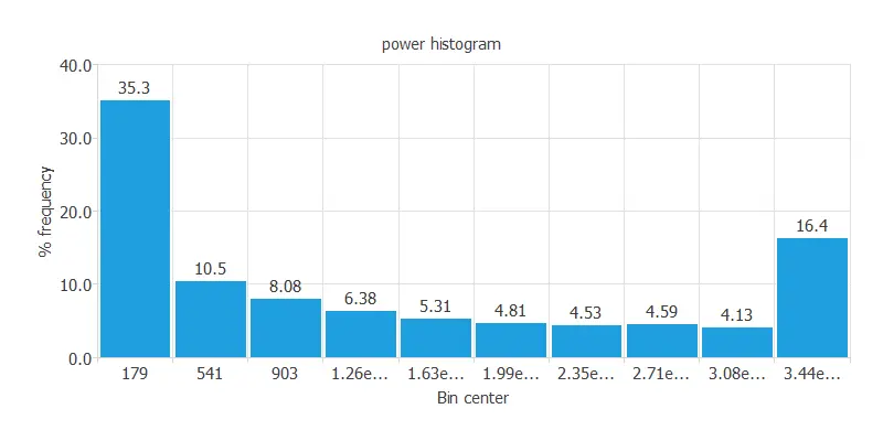
Calculating the data distributions helps us verify the accuracy of the available information and identify anomalies. The following chart shows the histogram for the power-generated variable:
It is also interesting to look for dependencies between input and target variables. To do that, we can calculate an input-targets correlation table.
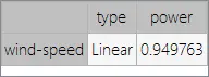
As expected, there is a high correlation between wind speed and the energy produced by the turbines.
Next, we plot a scatter chart.
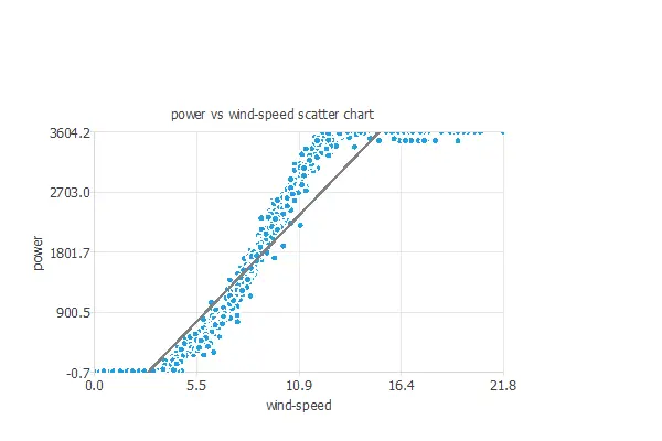
Here, we observe that the power generated increases linearly once a threshold wind level is surpassed until reaching an upper bound. Beyond this point, regardless of how much the wind speed exceeds the threshold, the power generated remains constant.
3. Neural network
The second step is to build a neural network that represents the approximation function. Approximation problems are typically composed of:
- Scaling layer.
- Perceptron layers.
- Unscaling layer.
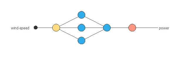
The neural network has 1 input (wind speed) and 1 output (power).
The scaling layer contains the statistics of the inputs. We use the automatic setting for this layer to accommodate the best scaling technique for our data.
We use 2 perceptron layers here:
- The first perceptron layer has 1 input, 3 neurons, and a hyperbolic tangent activation function.
- The second perceptron layer has 3 inputs, 1 neuron, and a linear activation function.
The unscaling layer contains the statistics of the outputs. We use the automatic method as before.
The next graph represents the neural network for this example.
4. Training strategy
The fourth step is to select an appropriate training strategy. It comprises two parameters:
- Loss index.
- Optimization algorithm.
The loss index defines what the neural network will learn. It comprises an error term and a regularization term.
We choose the normalized squared error as the error term. It divides the squared error between the neural network’s outputs and the targets in the data set by its normalization coefficient. If the normalized squared error has a value of 1, then the neural network is predicting the data ‘in the mean’, while a value of zero means a perfect prediction of the data. This error term does not have any parameters to set.
The regularization term is the L2 regularization. To control the neural network’s complexity, we adjust its parameters by reducing their values. We use a weak weight for this regularization term.
The optimization algorithm is responsible for searching for the neural network parameters that minimize the loss index. Here, we chose the quasi-Newton method as an optimization algorithm.
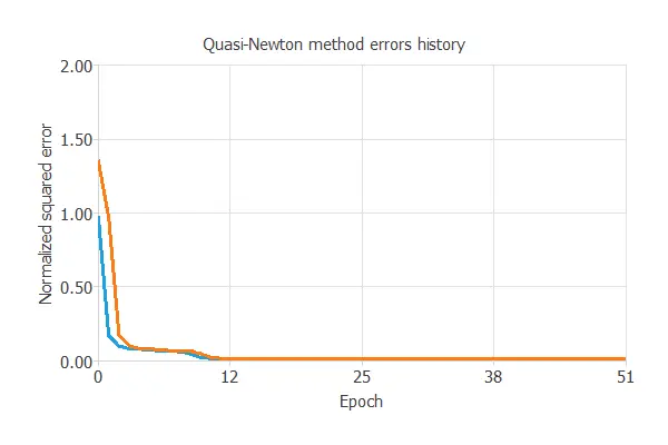
The following chart illustrates how the training (blue) and selection (orange) errors decrease with the number of epochs during the training process. The final values are training error = 0.00857 NSE and selection error = 0.00869 NSE, respectively.
5. Model selection
Model selection algorithms enhance the generalization performance of the neural network. As the selection error we have achieved so far is minimal (0.00869 NSE), this algorithm is unnecessary here.
6. Testing analysis
The purpose of the testing analysis is to validate the generalization capabilities of the neural network. We use the testing instances in the data set, which have never been used before.
A standard testing method in approximation applications is to perform a linear regression analysis between the predicted and the real pollutant level values.
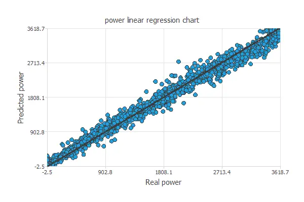
For a perfect fit, the correlation coefficient R2 would be 1. With R2 = 0.996, the neural network accurately predicts the testing data.
7. Model deployment
In the model deployment phase, the neural network is used to predict outputs for inputs that it has not seen before.
We can calculate the neural network outputs for a given set of inputs:
- wind-speed: 7.465 meters per second.
- power: 1166.580 kilowatts.
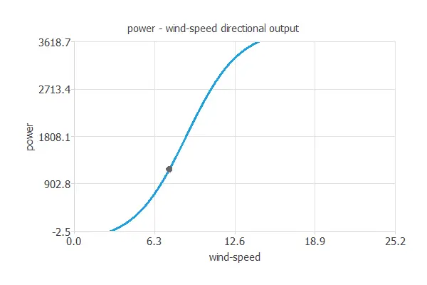
Directional outputs plot the neural network outputs through some reference points.
The reference point for the plot is the one we show next.
- wind-speed: 7.465 meters per second.
We can see here how the wind speed to solar noon affects the power generated:
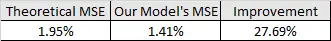
This application finds its true meaning when comparing the mean quadratic error of the fabricant’s calculations, using the theoretical turbine power equation (1.95%) versus our model’s error (1.41%), resulting in a 27.69% relative improvement.
Our model performs better because it considers the actual empirical data instead of a physical approximation.
The mathematical expression represented by the predictive model is displayed next:
scaled_wind-speed = wind-speed*(1+1)/(25.20599937-(0))-0*(1+1)/(25.20599937-0)-1;
perceptron_layer_output_0 = tanh[ -0.0837533 + (scaled_wind-speed*-0.297207) ];
perceptron_layer_output_1 = tanh[ -0.0199511 + (scaled_wind-speed*0.654869) ];
perceptron_layer_output_2 = tanh[ 0.811123 + (scaled_wind-speed*2.76357) ];
perceptron_layer_output_0 = [ -0.128215 + (perceptron_layer_output_0*0.290953)+ (perceptron_layer_output_1*-0.775739)+ (perceptron_layer_output_2*1.48548) ];
unscaling_layer_output_0 = perceptron_layer_output_0*(3618.72998+2.471410036)/(1+1)-2.471410036+1*(3618.72998+2.471410036)/(1+1);
8. Video tutorial
You can watch the step-by-step tutorial video below to help you complete this Machine Learning example
for free using the powerful machine learning software Neural Designer.
References
- Erisen, B. Wind Turbine Scada Dataset. 2018.