2. Data set
The first step is to prepare the data set, which is the source of information for the approximation problem. It consists of:
- Data source.
- Variables.
- Instances.
The file airfoil_self_noise.csv contains the data for this example. Here, the number of variables (columns) is 6, and the number of instances (rows) is 1503.
In that way, this problem has the 6 following variables:
- frequency, in Hertzs, used as input.
- angle_of_attack, in degrees, used as input.
- chord_length, in meters, used as input.
- free_stream_velocity, in meters per second, used as input.
- suction_side_displacement_thickness, in meters, used as input.
- scaled_sound_pressure_level, in decibels, used as the target.
On the other hand, the NASA data set contains 1503 instances. They are divided randomly into training, selection, and testing subsets, containing 60%, 20%, and 20% of the instances, respectively. More specifically, 753 samples are used here for training, 375 for validation, and 375 for testing.
Once all the data set information has been set, we will perform some analytics to check the quality of the data.
For instance, we can calculate the data distribution. The following figure depicts the histogram for the target variable.
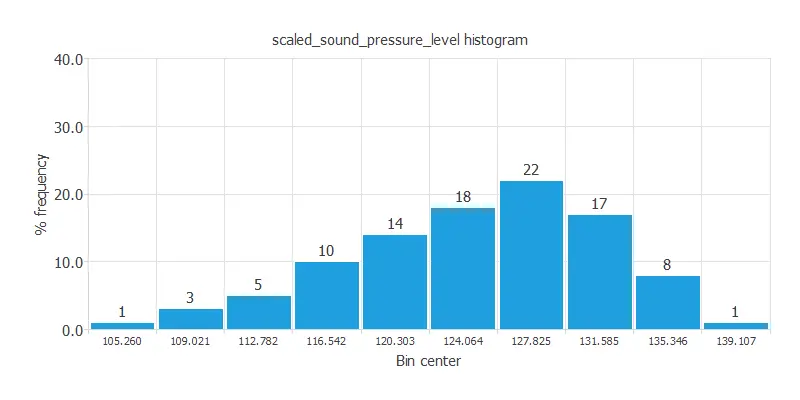
As we can see, the scaled sound pressure level has a normal distribution.
The following figure depicts inputs-targets correlations. This might help us see the different inputs’ influence on the sound level. As we can see, the wave’s frequency has the most significant impact on the noise.
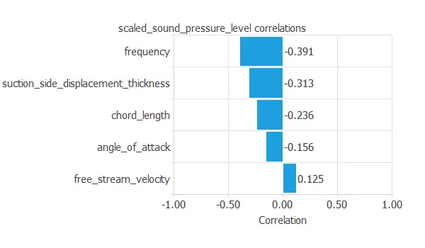
The above chart shows that the wave’s frequency has the most significant impact on the noise.
We can also plot a scatter chart with the scaled sound pressure level versus the frequency.
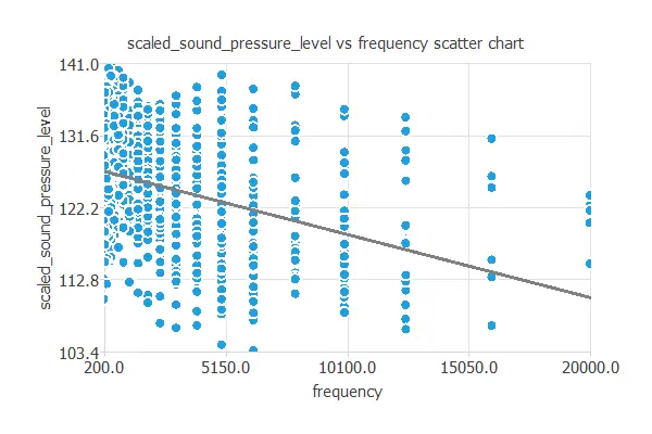
In general, the more frequency, the less scaled sound pressure level. However, the scaled sound pressure level depends on all the inputs simultaneously.
3. Neural network
The neural network will output the scaled sound pressure level as a function of the frequency, angle of attack, chord length, free stream velocity, and suction side displacement thickness.
For this approximation example, the neural network comprises:
- Scaling layer.
- Perceptron layers.
- Unscaling layer.
The scaling layer transforms the original inputs to normalized values. Here, the mean and standard deviation scaling method is set so that the input values have a mean of 0 and a standard deviation of 1.
Here two perceptron layers are added to the neural network. This number of layers is enough for most applications. The first layer has five inputs and three neurons. The second layer has three inputs and one neuron.
The unscaling layer transforms the normalized values from the neural network into the original outputs. Here, the mean and standard deviation unscaling method will also be used.
The next figure shows the resulting network architecture.
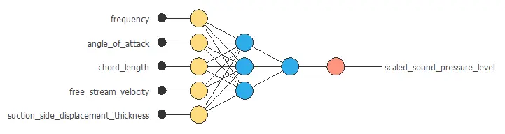
This neural network represents a function containing 22 adjustable parameters.
4. Training strategy
The next step is to select an appropriate training strategy, which defines what the neural network will learn. A general training strategy is composed of two concepts:
- A loss index.
- An optimization algorithm.
The loss index chosen is the normalized squared error with L2 regularization. This loss index is the default in approximation applications.
The optimization algorithm chosen is the quasi-Newton method. This optimization algorithm is the default for medium-sized applications like this one.
Once we have established the strategy, we can train the neural network. The following chart shows how the training (blue) and selection (orange) errors decrease with the training epoch during the training process.
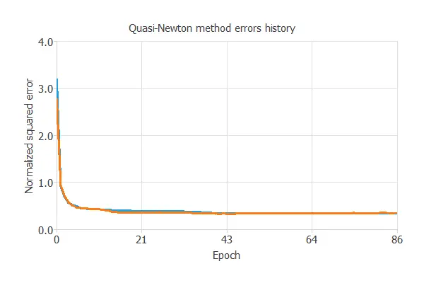
The most important training result is the final selection error. Indeed, this is a measure of the generalization capabilities of the neural network. Here the final selection error is selection error = 0.112 NSE.
5. Model selection
The objective of model selection is to find the network architecture with the best generalization properties. We want to improve the final selection error obtained before (0.112 NSE).
The best selection error is achieved using a model whose complexity is the most appropriate to produce an adequate data fit. Order selection algorithms are responsible for finding the optimal number of perceptrons in the neural network.
The following chart shows the results of the incremental order algorithm. The blue line plots the final training error as a function of the number of neurons, and the orange line plots the final selection error as a function of the number of neurons.
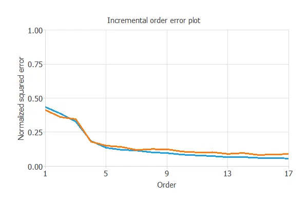
As we can see, the final training error always decreases with the number of neurons. However, the final selection error takes a minimum value at some point. Here, the optimal number of neurons is 13, corresponding to a selection error of 0.100 NSE.
The following figure shows the optimal network architecture for this application.
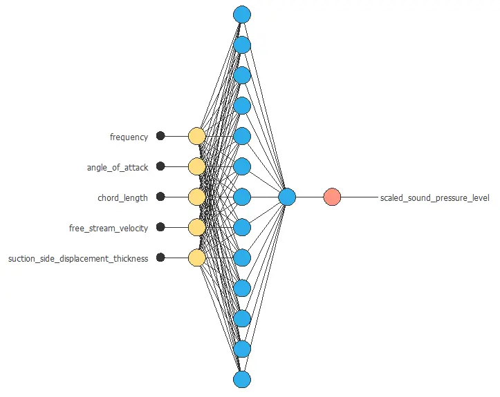
6. Testing analysis
The objective of the testing analysis is to validate the generalization performance of the trained neural network. The testing compares the values provided by this technique to the observed values.
A standard testing technique in approximation problems is to perform a linear regression analysis between the predicted and the real values,
using an independent testing set. The following figure illustrates a graphical output provided by this testing analysis.
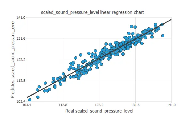
From the above chart, we can see that the neural network is predicting the entire range of sound level data well. The correlation value is R2 = 0.952, which is close to 1.
7. Model deployment
The model is ready to estimate the self-noise of new airfoils with satisfactory quality over the same data range.
We can now use Response Optimization. The objective of the response optimization algorithm is to exploit the mathematical model to look for optimal operating conditions. Indeed, the predictive model allows us to simulate different operating scenarios and adjust the control variables to improve efficiency.
An example is to maximize the speed while maintaining the sound pressure under the desired value.
The next table resumes the conditions for this problem.
| Variable name | Condition | |
|---|---|---|
| Frequency | None | |
| Angle of attack | None | |
| Chord length | None | |
| Free stream velocity | Maximize | |
| Suction side displacement thickness | None | |
| Scaled sound pressure level | Less than or equal to | 115 |
The next list shows the optimum values for previous conditions.
- frequency: 7087.22 Hertzs.
- angle_of_attack: 9.9381 degrees.
- chord_length: 0.206181 meters.
- free_stream_velocity: 71.1912 meters per second.
- suction_side_displacement_thickness: 0.015893 meters.
- scaled_sound_pressure_level: 108.015 decibels.
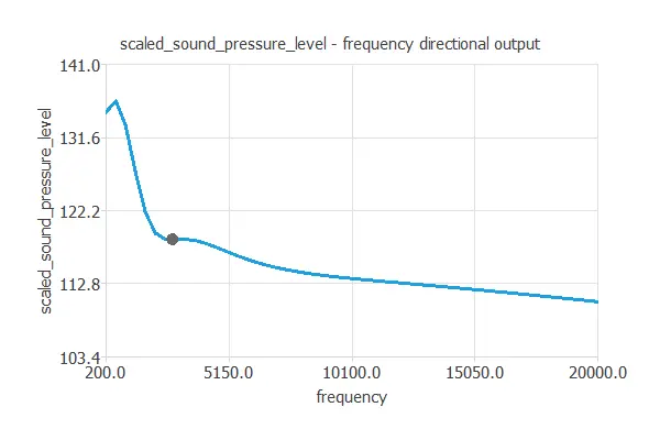
It is advantageous to see how the outputs vary as a single input function when all the others are fixed. Directional outputs plot the neural network outputs through some reference points.
The next list shows the reference points for the plots.
- angle_of_attack: 6.782 degrees.
- chord_length: 0.136 meters.
- free_stream_velocity: 50.860 meters per second.
- suction_side_displacement_thickness: 0.011 meters.
We can plot a directional output of the neural network to see how the sound level varies with a given input for all other fixed inputs. The next plot shows the sound level as a function of the frequency through the following point:
The file airfoil_self_noise.py contains the Python code for the scaled sound pressure level.