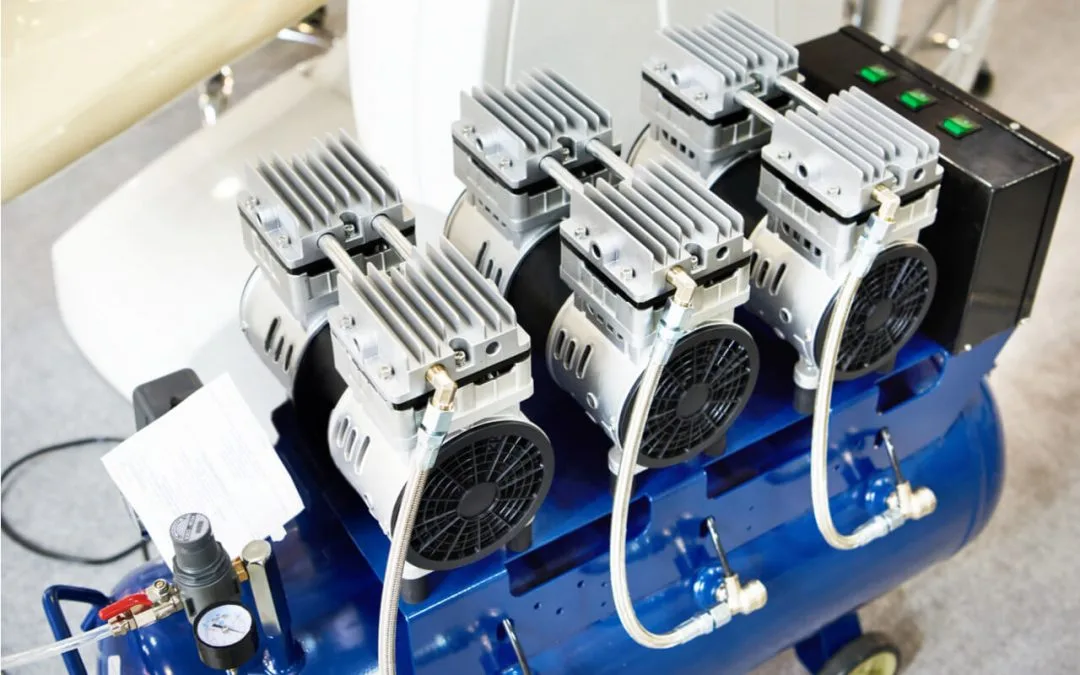
In this example, we build a machine learning model used as predictive maintenance to detect faults in an ultrasonic flow meter.
Predictive maintenance is a cutting-edge approach to equipment maintenance that utilizes data and analytics to predict when a machine or system is likely to fail.
By proactively identifying potential issues before they occur, businesses can save time and money and avoid costly downtime.
The occurrence of faults in public transport vehicles during their regular operation is a source of numerous damages, especially when they cause the interruption of the trip.
The negative impacts affect the operator company and the clients, who are disappointed with their expectations of transportation trust.
In this context, the early detection of such faults can avoid the cancellation of trips and the withdrawal of service from the respective vehicle and thus is of enormous value.
This example will explore a project with an urban metro public transportation service in Porto, Portugal.
The data, collected in 2022, aimed to evaluate machine learning methods for anomaly detection and failure prediction by capturing several analogic sensor signals (pressure, temperature, current consumption), digital signals (control signals, discrete signals), and GPS information (latitude, longitude, and speed), we provide a dataset that can be easily used to evaluate online machine learning methods.
Contents
- Application type.
- Data set.
- Neural network.
- Training strategy.
- Model selection.
- Testing analysis.
- Model deployment.
This example is solved with Neural Designer. To follow it step by step, you can use the free trial.
1. Application type
This is a classification project since the variable to be predicted is binary (healthy or unhealthy).
The goal is to model the probability that an ultrasonic flowmeter fails, conditioned on the process characteristics.
2. Dataset
The first step is to prepare the dataset, which is the source of information for the approximation problem.
It is composed of:
- Data source.
- Variables.
- Instances.
Data source
The file fault_detection.csv contains 87 instances of 37 diagnostic parameters corresponding to an 8-path liquid ultrasonic flow meter.
These 37 variables are all continuous except for the state of health.
Variables
The variables of the problem are:
- TP2: Measures the pressure on the compressor.
- TP3: Measures the pressure generated at the pneumatic panel.
- H1: This valve is activated when the pressure read by the pressure switch of the command is above the operating pressure of 10.2 bar.
- DV_pressure: Measures the pressure exerted due to the pressure drop generated when the air dryer towers discharge the water. When it is equal to zero, the compressor is working under load.
- Motor current: Measure the motor’s current, which should present the following values: (i) close to 0A when the compressor turns off; (ii) close to
4A when the compressor is working offloaded, and (iii) close to 7A when the compressor operates under load.
The digital sensors only assume two different values: zero when inactive or one when a specific event activates them. The considered digital sensors were the following:
- COMP: The electrical signal of the air intake valve on the compressor. It is active when there is no admission of air on the compressor, meaning that
the compressor turns off or is working offloaded. - DV electric: electrical signal that commands the compressor outlet valve. When it is active, it means that the compressor is working under load, and
when it is not active, it means that the compressor is off or working offloaded. - TOWERS: Defines which tower is drying the air and which is removing the humidity. When it is not active, it means that the tower
one is working, and when it is active, it means that tower two is working. - MPG: Activates the intake valve to start the compressor under load when the APU pressure is below 8.2 bar. Consequently, it
will activate the sensor COMP, which assumes the same behavior as the MPG sensor. - LPS: Is activated when the pressure is lower than 7 bars.
- Oil level: Detects the oil level on the compressor and is active (equal to one) when the oil is below the expected values.
Variables distributions
Once we have the prepared data, we will conduct a descriptive analysis of the problem to identify the key factors that should be considered in the training, thereby providing a logical and adequate solution to the problem.
We modify the most critical aspects during development, refining the solution to achieve the most precise and convenient outcome.
It is essential to know the ratio of negative and positive instances in the data set in the first place.
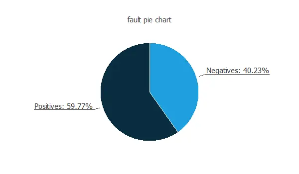
The chart shows that the number of negative instances (40.23%) and positive instances (59.77%) is similar.
This information will later be used to design the predictive model properly.
Inputs-targets correlations
The inputs-targets correlations shown in the next chart analyze the dependencies between each input variable and the target.
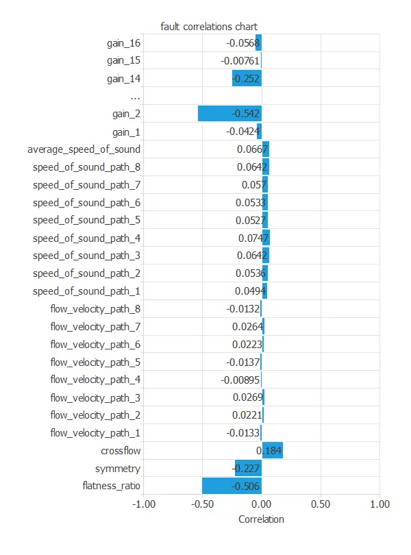
The flatness ratio (0.511) and some gains are most relevant to the target.
On the other hand, flow velocity in the paths contributes much less, so they are less determinant when deciding the state of health of the device.
The number of inputs is too high. Thus, we will set some input variables with a correlation with the target of less than 0,1 to unused variables. Furthermore, all gain variables will be manually set to input to build the model, considering all gains.
This data set contains 87 instances. From these, 53 instances are used for training (60%), 17 for generalization (20%), and 17 for testing (20%).
3. Neural network
The next step is to choose a neural network. For classification problems, it is usually composed of:
The scaling layer contains the statistics on the inputs calculated from the data file and the method for scaling the input variables.
Two perceptron layers with a hidden logistic layer and a logistic output layer are used. The neural network must have 19 inputs since these are the inputs selected after the descriptive analysis of the data. As an initial guess, we use three neurons in the hidden layer.
The probabilistic layer only contains the method for interpreting the outputs as probabilities. For this project, we set the binary probabilistic method as the target variable’s possible values 1 or 0.
The following figure shows the neural network structure that has been set for this data set.

4. Training strategy
The next step is to select an appropriate training strategy that defines what the neural network will learn. A general training strategy is composed of two concepts:
- A loss index.
- An optimization algorithm.
The data set is slightly unbalanced. Nevertheless, we use the normalized squared error with L2 regularization as the loss index.
Now, the model is ready to be trained. As the optimization algorithm, we use the default option for this type of case, the quasi-Newton method.
The following chart shows how training and selection errors decrease with the epochs during training.
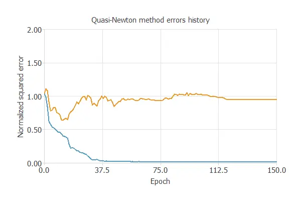
The final values are training error = 0.077 WSE and selection error = 1.07 WSE, respectively.
This selection error is not a reliable value. Therefore, to improve it, we must perform a model selection process.
5. Model selection
The objective of the model selection is to find the network architecture with the best generalization properties, that is, the one that minimizes the error on the selected instances of the data set.
More specifically, we want to find a neural network with a selection error of less than 1.07 WSE, the value we have achieved so far.
Order selection algorithms train several network architectures with a different number of neurons and select the one with the smallest selection error.
The incremental order method starts with a few neurons and increases the complexity at each iteration.
The following chart shows the training error (blue) and the selection error (orange) as a function of the number of neurons set for each iteration.
Besides, the new network architecture is represented below.
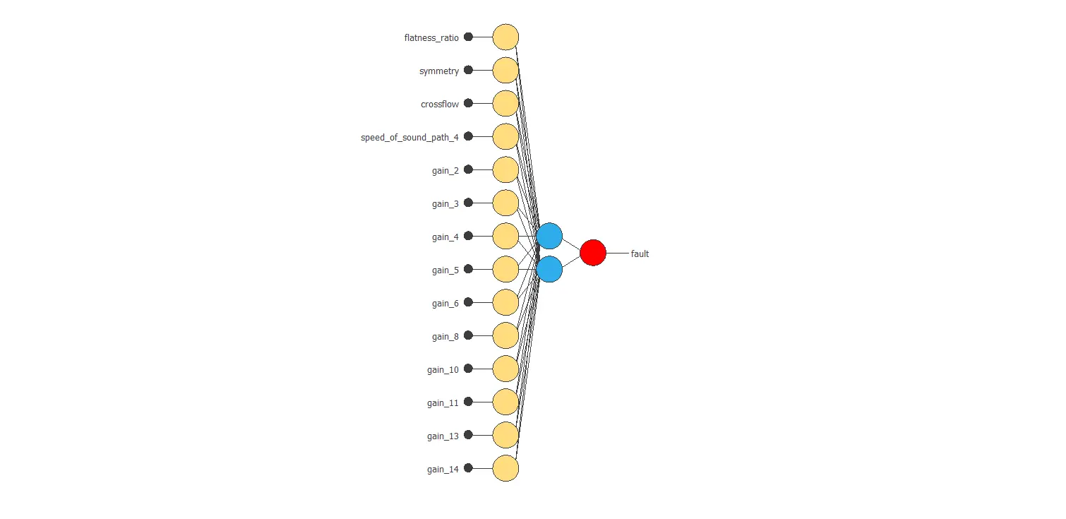
After the Order selection, the results are that the optimal network architecture consists of a single neuron in the perceptron layer. The selection error for this configuration is 0.41 WSE, which is far better than before.
6. Testing analysis
The testing analysis is responsible for evaluating the performance of our predictive model. First, we will check the ratio of positive and negative results from the outputs.
As shown in the above figure, the frequency for faulty meters is 47.058%, while for meters that work correctly, it is 52.941%.
The similarity in distribution is a good sign, as it is similar to the original dataset.
The ROC curve below is a good measure to check the precision of a binary classification model.
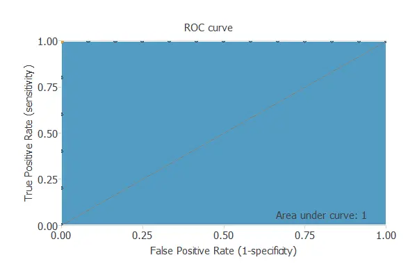
The parameter of importance here is the area under the curve (AUC). The value of this parameter must be higher than 0.5, and the closer to 1, the better. For this model, AUC = 0.764, which is not great but not random.
Another valid option to test the accuracy of a binary classification model is the confusion matrix. This matrix shows the number of negative and positive predicted values versus the real ones.
| Predicted positive | Predicted negative | |
|---|---|---|
| Real positive | 7 (41.2%) | 2 (11.8%) |
| Real negative | 2 (11.8%) | 6 (35.3%) |
From the confusion matrix, we can obtain the following binary classification tests:
- Accuracy (ratio of correctly classified samples): 76.5%
- Error (ratio of misclassified samples): 23.5%
- Sensitivity (percentage of actual positives classified as positive): 77.8%
- Specificity (percentage of actual negatives classified as negative): 75%
According to the results, our predictive model is slightly accurate (76.5%). The probability of success in positive cases is 77.8%, and in the negative cases, it is 75%, practically the same.
7. Model deployment
Once we know that our model is reliable and accurate, we can use it to check the health state of a meter, given the input variables’ required values.
This is called model deployment.
The predictive model provides a mathematical expression to integrate the function into other meters with the same variables.
Below is the mathematical expression:
scaled_flatness_ratio = (flatness_ratio-0.823907)/0.0182529;
scaled_symmetry = (symmetry-1.01097)/0.00580434;
scaled_crossflow = (crossflow-0.997436)/0.00202617;
scaled_gain_1 = (gain_1-33.9365)/0.240569;
scaled_gain_2 = (gain_2-33.3957)/0.0427105;
scaled_gain_3 = (gain_3-36.6963)/0.0213074;
scaled_gain_4 = (gain_4-36.8947)/0.107135;
scaled_gain_5 = (gain_5-35.1576)/0.0429498;
scaled_gain_6 = (gain_6-35.3841)/0.0959621;
scaled_gain_7 = (gain_7-33.537)/0.347826;
scaled_gain_8 = (gain_8-31.5031)/0.103171;
scaled_gain_9 = (gain_9-34.0167)/0.226074;
scaled_gain_10 = (gain_10-33.1856)/0.101873;
scaled_gain_11 = (gain_11-36.6672)/0.0195906;
scaled_gain_12 = (gain_12-36.7895)/0.0790561;
scaled_gain_13 = (gain_13-35.9453)/0.0577769;
scaled_gain_14 = (gain_14-35.9201)/0.0449897;
scaled_gain_15 = (gain_15-34.2524)/0.372388;
scaled_gain_16 = (gain_16-32.2916)/0.615941;
y_1_1 = Logistic (-0.25737+ (scaled_flatness_ratio*1.04101)+ (scaled_symmetry*-1.83364)+ (scaled_crossflow*7.42195)+ (scaled_gain_1*-2.34869)+ (scaled_gain_2*-8.03584)+ (scaled_gain_3*9.03579)+ (scaled_gain_4*-2.94732)+ (scaled_gain_5*-2.24593)+ (scaled_gain_6*-1.15397)+ (scaled_gain_7*5.47512)+ (scaled_gain_8*-4.10548)+ (scaled_gain_9*-1.91741)+ (scaled_gain_10*-4.7171)+ (scaled_gain_11*-0.496304)+ (scaled_gain_12*1.51573)+ (scaled_gain_13*-0.862037)+ (scaled_gain_14*-7.85136)+ (scaled_gain_15*0.977022)+ (scaled_gain_16*-3.77067));
non_probabilistic_fault = Logistic (-1.3648+ (y_1_1*9.12262));
fault = binary(non_probabilistic_fault);
logistic(x){
   return 1/(1+exp(-x))
}
binary(x){
   if x < decision_threshold
       return 0
   else
       return 1
}
For instance, one can export this expression to a dedicated engineering software used in the industry.
References:
- UCI Machine Learning Repository. Ultrasonic flowmeter diagnostics data set.
- K. S. Gyamfi, J. Brusey, A. Hunt, E. Gaura, Linear dimensionality reduction for classification via a sequential Bayes error minimisation with an application to flow meter diagnostics, Expert Systems with Applications (IF: 3.928), September 2017.