Explore the updated smartphone activity model
The current example includes 10,299 smartphone-signal feature rows with 561 inputs and six activity labels. Its saved configuration is available for inspection, but this .nd contains no completed task report.
1. Clinical question and intended use
A physiological-sensing workflow maps engineered smartphone-signal features to six activity categories. The current page documents the supplied data and network, without presenting performance from an earlier model as a result of this version.
Full feature set
Inspect all 561 recorded signal features.
Six activities
Retain the saved output-label order.
Evidence completion
Run and save the missing evaluation tasks.
2. Cohort, measurements and endpoint
The source is UCI Human Activity Recognition Using Smartphones. The adapted file contains the six labels LAYING, SITTING, STANDING, WALKING, WALKING_DOWNSTAIRS and WALKING_UPSTAIRS. The current model has 561 inputs, replacing the narrower feature table used by the former article.
Source: Human Activity Recognition Using Smartphones. Dataset license: CC-BY-4.0.
| Dataset measure | Saved value |
|---|---|
| Analysis unit | smartphone feature-window record |
| Records | 10,299 |
| Raw variables | 562 |
| Encoded model inputs | 561 |
| Model outputs | 6 |
| Training roles | 6181 |
| Validation / selection roles | 2059 |
| Testing roles | 2059 |
| Unused roles | 0 |
Inspect the complete saved variable schema
| Field | Role | Type | Categories |
|---|---|---|---|
| tBodyAcc_mean_X | Input | Numeric | |
| tBodyAcc_mean_Y | Input | Numeric | |
| tBodyAcc_mean_Z | Input | Numeric | |
| tBodyAcc_std_X | Input | Numeric | |
| tBodyAcc_std_Y | Input | Numeric | |
| tBodyAcc_std_Z | Input | Numeric | |
| tBodyAcc_mad_X | Input | Numeric | |
| tBodyAcc_mad_Y | Input | Numeric | |
| tBodyAcc_mad_Z | Input | Numeric | |
| tBodyAcc_max_X | Input | Numeric | |
| tBodyAcc_max_Y | Input | Numeric | |
| tBodyAcc_max_Z | Input | Numeric | |
| tBodyAcc_min_X | Input | Numeric | |
| tBodyAcc_min_Y | Input | Numeric | |
| tBodyAcc_min_Z | Input | Numeric | |
| tBodyAcc_sma | Input | Numeric | |
| tBodyAcc_energy_X | Input | Numeric | |
| tBodyAcc_energy_Y | Input | Numeric | |
| tBodyAcc_energy_Z | Input | Numeric | |
| tBodyAcc_iqr_X | Input | Numeric | |
| tBodyAcc_iqr_Y | Input | Numeric | |
| tBodyAcc_iqr_Z | Input | Numeric | |
| tBodyAcc_entropy_X | Input | Numeric | |
| tBodyAcc_entropy_Y | Input | Numeric | |
| tBodyAcc_entropy_Z | Input | Numeric | |
| tBodyAcc_arCoeff_X_1 | Input | Numeric | |
| tBodyAcc_arCoeff_X_2 | Input | Numeric | |
| tBodyAcc_arCoeff_X_3 | Input | Numeric | |
| tBodyAcc_arCoeff_X_4 | Input | Numeric | |
| tBodyAcc_arCoeff_Y_1 | Input | Numeric | |
| tBodyAcc_arCoeff_Y_2 | Input | Numeric | |
| tBodyAcc_arCoeff_Y_3 | Input | Numeric | |
| tBodyAcc_arCoeff_Y_4 | Input | Numeric | |
| tBodyAcc_arCoeff_Z_1 | Input | Numeric | |
| tBodyAcc_arCoeff_Z_2 | Input | Numeric | |
| tBodyAcc_arCoeff_Z_3 | Input | Numeric | |
| tBodyAcc_arCoeff_Z_4 | Input | Numeric | |
| tBodyAcc_correlation_X_Y | Input | Numeric | |
| tBodyAcc_correlation_X_Z | Input | Numeric | |
| tBodyAcc_correlation_Y_Z | Input | Numeric | |
| tGravityAcc_mean_X | Input | Numeric | |
| tGravityAcc_mean_Y | Input | Numeric | |
| tGravityAcc_mean_Z | Input | Numeric | |
| tGravityAcc_std_X | Input | Numeric | |
| tGravityAcc_std_Y | Input | Numeric | |
| tGravityAcc_std_Z | Input | Numeric | |
| tGravityAcc_mad_X | Input | Numeric | |
| tGravityAcc_mad_Y | Input | Numeric | |
| tGravityAcc_mad_Z | Input | Numeric | |
| tGravityAcc_max_X | Input | Numeric | |
| tGravityAcc_max_Y | Input | Numeric | |
| tGravityAcc_max_Z | Input | Numeric | |
| tGravityAcc_min_X | Input | Numeric | |
| tGravityAcc_min_Y | Input | Numeric | |
| tGravityAcc_min_Z | Input | Numeric | |
| tGravityAcc_sma | Input | Numeric | |
| tGravityAcc_energy_X | Input | Numeric | |
| tGravityAcc_energy_Y | Input | Numeric | |
| tGravityAcc_energy_Z | Input | Numeric | |
| tGravityAcc_iqr_X | Input | Numeric | |
| tGravityAcc_iqr_Y | Input | Numeric | |
| tGravityAcc_iqr_Z | Input | Numeric | |
| tGravityAcc_entropy_X | Input | Numeric | |
| tGravityAcc_entropy_Y | Input | Numeric | |
| tGravityAcc_entropy_Z | Input | Numeric | |
| tGravityAcc_arCoeff_X_1 | Input | Numeric | |
| tGravityAcc_arCoeff_X_2 | Input | Numeric | |
| tGravityAcc_arCoeff_X_3 | Input | Numeric | |
| tGravityAcc_arCoeff_X_4 | Input | Numeric | |
| tGravityAcc_arCoeff_Y_1 | Input | Numeric | |
| tGravityAcc_arCoeff_Y_2 | Input | Numeric | |
| tGravityAcc_arCoeff_Y_3 | Input | Numeric | |
| tGravityAcc_arCoeff_Y_4 | Input | Numeric | |
| tGravityAcc_arCoeff_Z_1 | Input | Numeric | |
| tGravityAcc_arCoeff_Z_2 | Input | Numeric | |
| tGravityAcc_arCoeff_Z_3 | Input | Numeric | |
| tGravityAcc_arCoeff_Z_4 | Input | Numeric | |
| tGravityAcc_correlation_X_Y | Input | Numeric | |
| tGravityAcc_correlation_X_Z | Input | Numeric | |
| tGravityAcc_correlation_Y_Z | Input | Numeric | |
| tBodyAccJerk_mean_X | Input | Numeric | |
| tBodyAccJerk_mean_Y | Input | Numeric | |
| tBodyAccJerk_mean_Z | Input | Numeric | |
| tBodyAccJerk_std_X | Input | Numeric | |
| tBodyAccJerk_std_Y | Input | Numeric | |
| tBodyAccJerk_std_Z | Input | Numeric | |
| tBodyAccJerk_mad_X | Input | Numeric | |
| tBodyAccJerk_mad_Y | Input | Numeric | |
| tBodyAccJerk_mad_Z | Input | Numeric | |
| tBodyAccJerk_max_X | Input | Numeric | |
| tBodyAccJerk_max_Y | Input | Numeric | |
| tBodyAccJerk_max_Z | Input | Numeric | |
| tBodyAccJerk_min_X | Input | Numeric | |
| tBodyAccJerk_min_Y | Input | Numeric | |
| tBodyAccJerk_min_Z | Input | Numeric | |
| tBodyAccJerk_sma | Input | Numeric | |
| tBodyAccJerk_energy_X | Input | Numeric | |
| tBodyAccJerk_energy_Y | Input | Numeric | |
| tBodyAccJerk_energy_Z | Input | Numeric | |
| tBodyAccJerk_iqr_X | Input | Numeric | |
| tBodyAccJerk_iqr_Y | Input | Numeric | |
| tBodyAccJerk_iqr_Z | Input | Numeric | |
| tBodyAccJerk_entropy_X | Input | Numeric | |
| tBodyAccJerk_entropy_Y | Input | Numeric | |
| tBodyAccJerk_entropy_Z | Input | Numeric | |
| tBodyAccJerk_arCoeff_X_1 | Input | Numeric | |
| tBodyAccJerk_arCoeff_X_2 | Input | Numeric | |
| tBodyAccJerk_arCoeff_X_3 | Input | Numeric | |
| tBodyAccJerk_arCoeff_X_4 | Input | Numeric | |
| tBodyAccJerk_arCoeff_Y_1 | Input | Numeric | |
| tBodyAccJerk_arCoeff_Y_2 | Input | Numeric | |
| tBodyAccJerk_arCoeff_Y_3 | Input | Numeric | |
| tBodyAccJerk_arCoeff_Y_4 | Input | Numeric | |
| tBodyAccJerk_arCoeff_Z_1 | Input | Numeric | |
| tBodyAccJerk_arCoeff_Z_2 | Input | Numeric | |
| tBodyAccJerk_arCoeff_Z_3 | Input | Numeric | |
| tBodyAccJerk_arCoeff_Z_4 | Input | Numeric | |
| tBodyAccJerk_correlation_X_Y | Input | Numeric | |
| tBodyAccJerk_correlation_X_Z | Input | Numeric | |
| tBodyAccJerk_correlation_Y_Z | Input | Numeric | |
| tBodyGyro_mean_X | Input | Numeric | |
| tBodyGyro_mean_Y | Input | Numeric | |
| tBodyGyro_mean_Z | Input | Numeric | |
| tBodyGyro_std_X | Input | Numeric | |
| tBodyGyro_std_Y | Input | Numeric | |
| tBodyGyro_std_Z | Input | Numeric | |
| tBodyGyro_mad_X | Input | Numeric | |
| tBodyGyro_mad_Y | Input | Numeric | |
| tBodyGyro_mad_Z | Input | Numeric | |
| tBodyGyro_max_X | Input | Numeric | |
| tBodyGyro_max_Y | Input | Numeric | |
| tBodyGyro_max_Z | Input | Numeric | |
| tBodyGyro_min_X | Input | Numeric | |
| tBodyGyro_min_Y | Input | Numeric | |
| tBodyGyro_min_Z | Input | Numeric | |
| tBodyGyro_sma | Input | Numeric | |
| tBodyGyro_energy_X | Input | Numeric | |
| tBodyGyro_energy_Y | Input | Numeric | |
| tBodyGyro_energy_Z | Input | Numeric | |
| tBodyGyro_iqr_X | Input | Numeric | |
| tBodyGyro_iqr_Y | Input | Numeric | |
| tBodyGyro_iqr_Z | Input | Numeric | |
| tBodyGyro_entropy_X | Input | Numeric | |
| tBodyGyro_entropy_Y | Input | Numeric | |
| tBodyGyro_entropy_Z | Input | Numeric | |
| tBodyGyro_arCoeff_X_1 | Input | Numeric | |
| tBodyGyro_arCoeff_X_2 | Input | Numeric | |
| tBodyGyro_arCoeff_X_3 | Input | Numeric | |
| tBodyGyro_arCoeff_X_4 | Input | Numeric | |
| tBodyGyro_arCoeff_Y_1 | Input | Numeric | |
| tBodyGyro_arCoeff_Y_2 | Input | Numeric | |
| tBodyGyro_arCoeff_Y_3 | Input | Numeric | |
| tBodyGyro_arCoeff_Y_4 | Input | Numeric | |
| tBodyGyro_arCoeff_Z_1 | Input | Numeric | |
| tBodyGyro_arCoeff_Z_2 | Input | Numeric | |
| tBodyGyro_arCoeff_Z_3 | Input | Numeric | |
| tBodyGyro_arCoeff_Z_4 | Input | Numeric | |
| tBodyGyro_correlation_X_Y | Input | Numeric | |
| tBodyGyro_correlation_X_Z | Input | Numeric | |
| tBodyGyro_correlation_Y_Z | Input | Numeric | |
| tBodyGyroJerk_mean_X | Input | Numeric | |
| tBodyGyroJerk_mean_Y | Input | Numeric | |
| tBodyGyroJerk_mean_Z | Input | Numeric | |
| tBodyGyroJerk_std_X | Input | Numeric | |
| tBodyGyroJerk_std_Y | Input | Numeric | |
| tBodyGyroJerk_std_Z | Input | Numeric | |
| tBodyGyroJerk_mad_X | Input | Numeric | |
| tBodyGyroJerk_mad_Y | Input | Numeric | |
| tBodyGyroJerk_mad_Z | Input | Numeric | |
| tBodyGyroJerk_max_X | Input | Numeric | |
| tBodyGyroJerk_max_Y | Input | Numeric | |
| tBodyGyroJerk_max_Z | Input | Numeric | |
| tBodyGyroJerk_min_X | Input | Numeric | |
| tBodyGyroJerk_min_Y | Input | Numeric | |
| tBodyGyroJerk_min_Z | Input | Numeric | |
| tBodyGyroJerk_sma | Input | Numeric | |
| tBodyGyroJerk_energy_X | Input | Numeric | |
| tBodyGyroJerk_energy_Y | Input | Numeric | |
| tBodyGyroJerk_energy_Z | Input | Numeric | |
| tBodyGyroJerk_iqr_X | Input | Numeric | |
| tBodyGyroJerk_iqr_Y | Input | Numeric | |
| tBodyGyroJerk_iqr_Z | Input | Numeric | |
| tBodyGyroJerk_entropy_X | Input | Numeric | |
| tBodyGyroJerk_entropy_Y | Input | Numeric | |
| tBodyGyroJerk_entropy_Z | Input | Numeric | |
| tBodyGyroJerk_arCoeff_X_1 | Input | Numeric | |
| tBodyGyroJerk_arCoeff_X_2 | Input | Numeric | |
| tBodyGyroJerk_arCoeff_X_3 | Input | Numeric | |
| tBodyGyroJerk_arCoeff_X_4 | Input | Numeric | |
| tBodyGyroJerk_arCoeff_Y_1 | Input | Numeric | |
| tBodyGyroJerk_arCoeff_Y_2 | Input | Numeric | |
| tBodyGyroJerk_arCoeff_Y_3 | Input | Numeric | |
| tBodyGyroJerk_arCoeff_Y_4 | Input | Numeric | |
| tBodyGyroJerk_arCoeff_Z_1 | Input | Numeric | |
| tBodyGyroJerk_arCoeff_Z_2 | Input | Numeric | |
| tBodyGyroJerk_arCoeff_Z_3 | Input | Numeric | |
| tBodyGyroJerk_arCoeff_Z_4 | Input | Numeric | |
| tBodyGyroJerk_correlation_X_Y | Input | Numeric | |
| tBodyGyroJerk_correlation_X_Z | Input | Numeric | |
| tBodyGyroJerk_correlation_Y_Z | Input | Numeric | |
| tBodyAccMag_mean | Input | Numeric | |
| tBodyAccMag_std | Input | Numeric | |
| tBodyAccMag_mad | Input | Numeric | |
| tBodyAccMag_max | Input | Numeric | |
| tBodyAccMag_min | Input | Numeric | |
| tBodyAccMag_sma | Input | Numeric | |
| tBodyAccMag_energy | Input | Numeric | |
| tBodyAccMag_iqr | Input | Numeric | |
| tBodyAccMag_entropy | Input | Numeric | |
| tBodyAccMag_arCoeff1 | Input | Numeric | |
| tBodyAccMag_arCoeff2 | Input | Numeric | |
| tBodyAccMag_arCoeff3 | Input | Numeric | |
| tBodyAccMag_arCoeff4 | Input | Numeric | |
| tGravityAccMag_mean | Input | Numeric | |
| tGravityAccMag_std | Input | Numeric | |
| tGravityAccMag_mad | Input | Numeric | |
| tGravityAccMag_max | Input | Numeric | |
| tGravityAccMag_min | Input | Numeric | |
| tGravityAccMag_sma | Input | Numeric | |
| tGravityAccMag_energy | Input | Numeric | |
| tGravityAccMag_iqr | Input | Numeric | |
| tGravityAccMag_entropy | Input | Numeric | |
| tGravityAccMag_arCoeff1 | Input | Numeric | |
| tGravityAccMag_arCoeff2 | Input | Numeric | |
| tGravityAccMag_arCoeff3 | Input | Numeric | |
| tGravityAccMag_arCoeff4 | Input | Numeric | |
| tBodyAccJerkMag_mean | Input | Numeric | |
| tBodyAccJerkMag_std | Input | Numeric | |
| tBodyAccJerkMag_mad | Input | Numeric | |
| tBodyAccJerkMag_max | Input | Numeric | |
| tBodyAccJerkMag_min | Input | Numeric | |
| tBodyAccJerkMag_sma | Input | Numeric | |
| tBodyAccJerkMag_energy | Input | Numeric | |
| tBodyAccJerkMag_iqr | Input | Numeric | |
| tBodyAccJerkMag_entropy | Input | Numeric | |
| tBodyAccJerkMag_arCoeff1 | Input | Numeric | |
| tBodyAccJerkMag_arCoeff2 | Input | Numeric | |
| tBodyAccJerkMag_arCoeff3 | Input | Numeric | |
| tBodyAccJerkMag_arCoeff4 | Input | Numeric | |
| tBodyGyroMag_mean | Input | Numeric | |
| tBodyGyroMag_std | Input | Numeric | |
| tBodyGyroMag_mad | Input | Numeric | |
| tBodyGyroMag_max | Input | Numeric | |
| tBodyGyroMag_min | Input | Numeric | |
| tBodyGyroMag_sma | Input | Numeric | |
| tBodyGyroMag_energy | Input | Numeric | |
| tBodyGyroMag_iqr | Input | Numeric | |
| tBodyGyroMag_entropy | Input | Numeric | |
| tBodyGyroMag_arCoeff1 | Input | Numeric | |
| tBodyGyroMag_arCoeff2 | Input | Numeric | |
| tBodyGyroMag_arCoeff3 | Input | Numeric | |
| tBodyGyroMag_arCoeff4 | Input | Numeric | |
| tBodyGyroJerkMag_mean | Input | Numeric | |
| tBodyGyroJerkMag_std | Input | Numeric | |
| tBodyGyroJerkMag_mad | Input | Numeric | |
| tBodyGyroJerkMag_max | Input | Numeric | |
| tBodyGyroJerkMag_min | Input | Numeric | |
| tBodyGyroJerkMag_sma | Input | Numeric | |
| tBodyGyroJerkMag_energy | Input | Numeric | |
| tBodyGyroJerkMag_iqr | Input | Numeric | |
| tBodyGyroJerkMag_entropy | Input | Numeric | |
| tBodyGyroJerkMag_arCoeff1 | Input | Numeric | |
| tBodyGyroJerkMag_arCoeff2 | Input | Numeric | |
| tBodyGyroJerkMag_arCoeff3 | Input | Numeric | |
| tBodyGyroJerkMag_arCoeff4 | Input | Numeric | |
| fBodyAcc_mean_X | Input | Numeric | |
| fBodyAcc_mean_Y | Input | Numeric | |
| fBodyAcc_mean_Z | Input | Numeric | |
| fBodyAcc_std_X | Input | Numeric | |
| fBodyAcc_std_Y | Input | Numeric | |
| fBodyAcc_std_Z | Input | Numeric | |
| fBodyAcc_mad_X | Input | Numeric | |
| fBodyAcc_mad_Y | Input | Numeric | |
| fBodyAcc_mad_Z | Input | Numeric | |
| fBodyAcc_max_X | Input | Numeric | |
| fBodyAcc_max_Y | Input | Numeric | |
| fBodyAcc_max_Z | Input | Numeric | |
| fBodyAcc_min_X | Input | Numeric | |
| fBodyAcc_min_Y | Input | Numeric | |
| fBodyAcc_min_Z | Input | Numeric | |
| fBodyAcc_sma | Input | Numeric | |
| fBodyAcc_energy_X | Input | Numeric | |
| fBodyAcc_energy_Y | Input | Numeric | |
| fBodyAcc_energy_Z | Input | Numeric | |
| fBodyAcc_iqr_X | Input | Numeric | |
| fBodyAcc_iqr_Y | Input | Numeric | |
| fBodyAcc_iqr_Z | Input | Numeric | |
| fBodyAcc_entropy_X | Input | Numeric | |
| fBodyAcc_entropy_Y | Input | Numeric | |
| fBodyAcc_entropy_Z | Input | Numeric | |
| fBodyAcc_maxInds_X | Input | Numeric | |
| fBodyAcc_maxInds_Y | Input | Numeric | |
| fBodyAcc_maxInds_Z | Input | Numeric | |
| fBodyAcc_meanFreq_X | Input | Numeric | |
| fBodyAcc_meanFreq_Y | Input | Numeric | |
| fBodyAcc_meanFreq_Z | Input | Numeric | |
| fBodyAcc_skewness_X | Input | Numeric | |
| fBodyAcc_kurtosis_X | Input | Numeric | |
| fBodyAcc_skewness_Y | Input | Numeric | |
| fBodyAcc_kurtosis_Y | Input | Numeric | |
| fBodyAcc_skewness_Z | Input | Numeric | |
| fBodyAcc_kurtosis_Z | Input | Numeric | |
| fBodyAcc_bandsEnergy_1_8 | Input | Numeric | |
| fBodyAcc_bandsEnergy_9_16 | Input | Numeric | |
| fBodyAcc_bandsEnergy_17_24 | Input | Numeric | |
| fBodyAcc_bandsEnergy_25_32 | Input | Numeric | |
| fBodyAcc_bandsEnergy_33_40 | Input | Numeric | |
| fBodyAcc_bandsEnergy_41_48 | Input | Numeric | |
| fBodyAcc_bandsEnergy_49_56 | Input | Numeric | |
| fBodyAcc_bandsEnergy_57_64 | Input | Numeric | |
| fBodyAcc_bandsEnergy_1_16 | Input | Numeric | |
| fBodyAcc_bandsEnergy_17_32 | Input | Numeric | |
| fBodyAcc_bandsEnergy_33_48 | Input | Numeric | |
| fBodyAcc_bandsEnergy_49_64 | Input | Numeric | |
| fBodyAcc_bandsEnergy_1_24 | Input | Numeric | |
| fBodyAcc_bandsEnergy_25_48 | Input | Numeric | |
| fBodyAcc_bandsEnergy_1_8 | Input | Numeric | |
| fBodyAcc_bandsEnergy_9_16 | Input | Numeric | |
| fBodyAcc_bandsEnergy_17_24 | Input | Numeric | |
| fBodyAcc_bandsEnergy_25_32 | Input | Numeric | |
| fBodyAcc_bandsEnergy_33_40 | Input | Numeric | |
| fBodyAcc_bandsEnergy_41_48 | Input | Numeric | |
| fBodyAcc_bandsEnergy_49_56 | Input | Numeric | |
| fBodyAcc_bandsEnergy_57_64 | Input | Numeric | |
| fBodyAcc_bandsEnergy_1_16 | Input | Numeric | |
| fBodyAcc_bandsEnergy_17_32 | Input | Numeric | |
| fBodyAcc_bandsEnergy_33_48 | Input | Numeric | |
| fBodyAcc_bandsEnergy_49_64 | Input | Numeric | |
| fBodyAcc_bandsEnergy_1_24 | Input | Numeric | |
| fBodyAcc_bandsEnergy_25_48 | Input | Numeric | |
| fBodyAcc_bandsEnergy_1_8 | Input | Numeric | |
| fBodyAcc_bandsEnergy_9_16 | Input | Numeric | |
| fBodyAcc_bandsEnergy_17_24 | Input | Numeric | |
| BodyAcc_bandsEnergy_25_32 | Input | Numeric | |
| fBodyAcc_bandsEnergy_33_40 | Input | Numeric | |
| fBodyAcc_bandsEnergy_41_48 | Input | Numeric | |
| fBodyAcc_bandsEnergy_49_56 | Input | Numeric | |
| fBodyAcc_bandsEnergy_57_64 | Input | Numeric | |
| fBodyAcc_bandsEnergy_1_16 | Input | Numeric | |
| fBodyAcc_bandsEnergy_17_32 | Input | Numeric | |
| fBodyAcc_bandsEnergy_33_48 | Input | Numeric | |
| fBodyAcc_bandsEnergy_49_64 | Input | Numeric | |
| fBodyAcc_bandsEnergy_1_24 | Input | Numeric | |
| fBodyAcc_bandsEnergy_25_48 | Input | Numeric | |
| fBodyAccJerk_mean_X | Input | Numeric | |
| fBodyAccJerk_mean_Y | Input | Numeric | |
| fBodyAccJerk_mean_Z | Input | Numeric | |
| fBodyAccJerk_std_X | Input | Numeric | |
| fBodyAccJerk_std_Y | Input | Numeric | |
| fBodyAccJerk_std_Z | Input | Numeric | |
| fBodyAccJerk_mad_X | Input | Numeric | |
| fBodyAccJerk_mad_Y | Input | Numeric | |
| fBodyAccJerk_mad_Z | Input | Numeric | |
| fBodyAccJerk_max_X | Input | Numeric | |
| fBodyAccJerk_max_Y | Input | Numeric | |
| fBodyAccJerk_max_Z | Input | Numeric | |
| fBodyAccJerk_min_X | Input | Numeric | |
| fBodyAccJerk_min_Y | Input | Numeric | |
| fBodyAccJerk_min_Z | Input | Numeric | |
| fBodyAccJerk_sma | Input | Numeric | |
| fBodyAccJerk_energy_X | Input | Numeric | |
| fBodyAccJerk_energy_Y | Input | Numeric | |
| fBodyAccJerk_energy_Z | Input | Numeric | |
| fBodyAccJerk_iqr_X | Input | Numeric | |
| fBodyAccJerk_iqr_Y | Input | Numeric | |
| fBodyAccJerk_iqr_Z | Input | Numeric | |
| fBodyAccJerk_entropy_X | Input | Numeric | |
| fBodyAccJerk_entropy_Y | Input | Numeric | |
| fBodyAccJerk_entropy_Z | Input | Numeric | |
| fBodyAccJerk_maxInds_X | Input | Numeric | |
| fBodyAccJerk_maxInds_Y | Input | Numeric | |
| fBodyAccJerk_maxInds_Z | Input | Numeric | |
| fBodyAccJerk_meanFreq_X | Input | Numeric | |
| fBodyAccJerk_meanFreq_Y | Input | Numeric | |
| fBodyAccJerk_meanFreq_Z | Input | Numeric | |
| fBodyAccJerk_skewness_X | Input | Numeric | |
| fBodyAccJerk_kurtosis_X | Input | Numeric | |
| fBodyAccJerk_skewness_Y | Input | Numeric | |
| fBodyAccJerk_kurtosis_Y | Input | Numeric | |
| fBodyAccJerk_skewness_Z | Input | Numeric | |
| fBodyAccJerk_kurtosis_Z | Input | Numeric | |
| fBodyAccJerk_bandsEnergy_1_8 | Input | Numeric | |
| fBodyAccJerk_bandsEnergy_9_16 | Input | Numeric | |
| fBodyAccJerk_bandsEnergy_17_24 | Input | Numeric | |
| fBodyAccJerk_bandsEnergy_25_32 | Input | Numeric | |
| fBodyAccJerk_bandsEnergy_33_40 | Input | Numeric | |
| fBodyAccJerk_bandsEnergy_41_48 | Input | Numeric | |
| fBodyAccJerk_bandsEnergy_49_56 | Input | Numeric | |
| fBodyAccJerk_bandsEnergy_57_64 | Input | Numeric | |
| fBodyAccJerk_bandsEnergy_1_16 | Input | Numeric | |
| fBodyAccJerk_bandsEnergy_17_32 | Input | Numeric | |
| fBodyAccJerk_bandsEnergy_33_48 | Input | Numeric | |
| fBodyAccJerk_bandsEnergy_49_64 | Input | Numeric | |
| fBodyAccJerk_bandsEnergy_1_24 | Input | Numeric | |
| fBodyAccJerk_bandsEnergy_25_48 | Input | Numeric | |
| fBodyAccJerk_bandsEnergy_1_8 | Input | Numeric | |
| fBodyAccJerk_bandsEnergy_9_16 | Input | Numeric | |
| fBodyAccJerk_bandsEnergy_17_24 | Input | Numeric | |
| fBodyAccJerk_bandsEnergy_25_32 | Input | Numeric | |
| fBodyAccJerk_bandsEnergy_33_40 | Input | Numeric | |
| fBodyAccJerk_bandsEnergy_41_48 | Input | Numeric | |
| fBodyAccJerk_bandsEnergy_49_56 | Input | Numeric | |
| fBodyAccJerk_bandsEnergy_57_64 | Input | Numeric | |
| fBodyAccJerk_bandsEnergy_1_16 | Input | Numeric | |
| fBodyAccJerk_bandsEnergy_17_32 | Input | Numeric | |
| fBodyAccJerk_bandsEnergy_33_48 | Input | Numeric | |
| fBodyAccJerk_bandsEnergy_49_64 | Input | Numeric | |
| fBodyAccJerk_bandsEnergy_1_24 | Input | Numeric | |
| fBodyAccJerk_bandsEnergy_25_48 | Input | Numeric | |
| fBodyAccJerk_bandsEnergy_1_8 | Input | Numeric | |
| fBodyAccJerk_bandsEnergy_9_16 | Input | Numeric | |
| fBodyAccJerk_bandsEnergy_17_24 | Input | Numeric | |
| fBodyAccJerk_bandsEnergy_25_32 | Input | Numeric | |
| fBodyAccJerk_bandsEnergy_33_40 | Input | Numeric | |
| fBodyAccJerk_bandsEnergy_41_48 | Input | Numeric | |
| fBodyAccJerk_bandsEnergy_49_56 | Input | Numeric | |
| fBodyAccJerk_bandsEnergy_57_64 | Input | Numeric | |
| fBodyAccJerk_bandsEnergy_1_16 | Input | Numeric | |
| fBodyAccJerk_bandsEnergy_17_32 | Input | Numeric | |
| fBodyAccJerk_bandsEnergy_33_48 | Input | Numeric | |
| fBodyAccJerk_bandsEnergy_49_64 | Input | Numeric | |
| fBodyAccJerk_bandsEnergy_1_24 | Input | Numeric | |
| fBodyAccJerk_bandsEnergy_25_48 | Input | Numeric | |
| fBodyGyro_mean_X | Input | Numeric | |
| fBodyGyro_mean_Y | Input | Numeric | |
| fBodyGyro_mean_Z | Input | Numeric | |
| fBodyGyro_std_X | Input | Numeric | |
| fBodyGyro_std_Y | Input | Numeric | |
| fBodyGyro_std_Z | Input | Numeric | |
| fBodyGyro_mad_X | Input | Numeric | |
| fBodyGyro_mad_Y | Input | Numeric | |
| fBodyGyro_mad_Z | Input | Numeric | |
| fBodyGyro_max_X | Input | Numeric | |
| fBodyGyro_max_Y | Input | Numeric | |
| fBodyGyro_max_Z | Input | Numeric | |
| fBodyGyro_min_X | Input | Numeric | |
| fBodyGyro_min_Y | Input | Numeric | |
| fBodyGyro_min_Z | Input | Numeric | |
| fBodyGyro_sma | Input | Numeric | |
| fBodyGyro_energy_X | Input | Numeric | |
| fBodyGyro_energy_Y | Input | Numeric | |
| fBodyGyro_energy_Z | Input | Numeric | |
| fBodyGyro_iqr_X | Input | Numeric | |
| fBodyGyro_iqr_Y | Input | Numeric | |
| fBodyGyro_iqr_Z | Input | Numeric | |
| fBodyGyro_entropy_X | Input | Numeric | |
| fBodyGyro_entropy_Y | Input | Numeric | |
| fBodyGyro_entropy_Z | Input | Numeric | |
| fBodyGyro_maxInds_X | Input | Numeric | |
| fBodyGyro_maxInds_Y | Input | Numeric | |
| fBodyGyro_maxInds_Z | Input | Numeric | |
| fBodyGyro_meanFreq_X | Input | Numeric | |
| fBodyGyro_meanFreq_Y | Input | Numeric | |
| fBodyGyro_meanFreq_Z | Input | Numeric | |
| fBodyGyro_skewness_X | Input | Numeric | |
| fBodyGyro_kurtosis_X | Input | Numeric | |
| fBodyGyro_skewness_Y | Input | Numeric | |
| fBodyGyro_kurtosis_Y | Input | Numeric | |
| fBodyGyro_skewness_Z | Input | Numeric | |
| fBodyGyro_kurtosis_Z | Input | Numeric | |
| fBodyGyro_bandsEnergy_1_8 | Input | Numeric | |
| fBodyGyro_bandsEnergy_9_16 | Input | Numeric | |
| fBodyGyro_bandsEnergy_17_24 | Input | Numeric | |
| fBodyGyro_bandsEnergy_25_32 | Input | Numeric | |
| fBodyGyro_bandsEnergy_33_40 | Input | Numeric | |
| fBodyGyro_bandsEnergy_41_48 | Input | Numeric | |
| fBodyGyro_bandsEnergy_49_56 | Input | Numeric | |
| fBodyGyro_bandsEnergy_57_64 | Input | Numeric | |
| fBodyGyro_bandsEnergy_1_16 | Input | Numeric | |
| fBodyGyro_bandsEnergy_17_32 | Input | Numeric | |
| fBodyGyro_bandsEnergy_33_48 | Input | Numeric | |
| fBodyGyro_bandsEnergy_49_64 | Input | Numeric | |
| fBodyGyro_bandsEnergy_1_24 | Input | Numeric | |
| fBodyGyro_bandsEnergy_25_48 | Input | Numeric | |
| fBodyGyro_bandsEnergy_1_8 | Input | Numeric | |
| fBodyGyro_bandsEnergy_9_16 | Input | Numeric | |
| fBodyGyro_bandsEnergy_17_24 | Input | Numeric | |
| fBodyGyro_bandsEnergy_25_32 | Input | Numeric | |
| fBodyGyro_bandsEnergy_33_40 | Input | Numeric | |
| fBodyGyro_bandsEnergy_41_48 | Input | Numeric | |
| fBodyGyro_bandsEnergy_49_56 | Input | Numeric | |
| fBodyGyro_bandsEnergy_57_64 | Input | Numeric | |
| fBodyGyro_bandsEnergy_1_16 | Input | Numeric | |
| fBodyGyro_bandsEnergy_17_32 | Input | Numeric | |
| fBodyGyro_bandsEnergy_33_48 | Input | Numeric | |
| fBodyGyro_bandsEnergy_49_64 | Input | Numeric | |
| fBodyGyro_bandsEnergy_1_24 | Input | Numeric | |
| fBodyGyro_bandsEnergy_25_48 | Input | Numeric | |
| fBodyGyro_bandsEnergy_1_8 | Input | Numeric | |
| fBodyGyro_bandsEnergy_9_16 | Input | Numeric | |
| fBodyGyro_bandsEnergy_17_24 | Input | Numeric | |
| fBodyGyro_bandsEnergy_25_32 | Input | Numeric | |
| fBodyGyro_bandsEnergy_33_40 | Input | Numeric | |
| fBodyGyro_bandsEnergy_41_48 | Input | Numeric | |
| fBodyGyro_bandsEnergy_49_56 | Input | Numeric | |
| fBodyGyro_bandsEnergy_57_64 | Input | Numeric | |
| fBodyGyro_bandsEnergy_1_16 | Input | Numeric | |
| fBodyGyro_bandsEnergy_17_32 | Input | Numeric | |
| fBodyGyro_bandsEnergy_33_48 | Input | Numeric | |
| fBodyGyro_bandsEnergy_49_64 | Input | Numeric | |
| fBodyGyro_bandsEnergy_1_24 | Input | Numeric | |
| fBodyGyro_bandsEnergy_25_48 | Input | Numeric | |
| fBodyAccMag_mean | Input | Numeric | |
| fBodyAccMag_std | Input | Numeric | |
| fBodyAccMag_mad | Input | Numeric | |
| fBodyAccMag_max | Input | Numeric | |
| fBodyAccMag_min | Input | Numeric | |
| fBodyAccMag_sma | Input | Numeric | |
| fBodyAccMag_energy | Input | Numeric | |
| fBodyAccMag_iqr | Input | Numeric | |
| BodyAccMag_entropy | Input | Numeric | |
| fBodyAccMag_maxInds | Input | Numeric | |
| fBodyAccMag_meanFreq | Input | Numeric | |
| fBodyAccMag_skewness | Input | Numeric | |
| fBodyAccMag_kurtosis | Input | Numeric | |
| fBodyBodyAccJerkMag_mean | Input | Numeric | |
| fBodyBodyAccJerkMag_std | Input | Numeric | |
| fBodyBodyAccJerkMag_mad | Input | Numeric | |
| fBodyBodyAccJerkMag_max | Input | Numeric | |
| fBodyBodyAccJerkMag_min | Input | Numeric | |
| fBodyBodyAccJerkMag_sma | Input | Numeric | |
| fBodyBodyAccJerkMag_energy | Input | Numeric | |
| fBodyBodyAccJerkMag_iqr | Input | Numeric | |
| fBodyBodyAccJerkMag_entropy | Input | Numeric | |
| fBodyBodyAccJerkMag_maxInds | Input | Numeric | |
| fBodyBodyAccJerkMag_meanFreq | Input | Numeric | |
| fBodyBodyAccJerkMag_skewness | Input | Numeric | |
| fBodyBodyAccJerkMag_kurtosis | Input | Numeric | |
| fBodyBodyGyroMag_mean | Input | Numeric | |
| fBodyBodyGyroMag_std | Input | Numeric | |
| fBodyBodyGyroMag_mad | Input | Numeric | |
| fBodyBodyGyroMag_max | Input | Numeric | |
| fBodyBodyGyroMag_min | Input | Numeric | |
| fBodyBodyGyroMag_sma | Input | Numeric | |
| fBodyBodyGyroMag_energy | Input | Numeric | |
| fBodyBodyGyroMag_iqr | Input | Numeric | |
| fBodyBodyGyroMag_entropy | Input | Numeric | |
| fBodyBodyGyroMag_maxInds | Input | Numeric | |
| fBodyBodyGyroMag_meanFreq | Input | Numeric | |
| fBodyBodyGyroMag_skewness | Input | Numeric | |
| fBodyBodyGyroMag_kurtosis | Input | Numeric | |
| fBodyBodyGyroJerkMag_mean | Input | Numeric | |
| fBodyBodyGyroJerkMag_std | Input | Numeric | |
| fBodyBodyGyroJerkMag_mad | Input | Numeric | |
| fBodyBodyGyroJerkMag_max | Input | Numeric | |
| fBodyBodyGyroJerkMag_min | Input | Numeric | |
| fBodyBodyGyroJerkMag_sma | Input | Numeric | |
| fBodyBodyGyroJerkMag_energy | Input | Numeric | |
| fBodyBodyGyroJerkMag_iqr | Input | Numeric | |
| fBodyBodyGyroJerkMag_entropy | Input | Numeric | |
| fBodyBodyGyroJerkMag_maxInds | Input | Numeric | |
| fBodyBodyGyroJerkMag_meanFreq | Input | Numeric | |
| fBodyBodyGyroJerkMag_skewness | Input | Numeric | |
| fBodyBodyGyroJerkMag_kurtosis | Input | Numeric | |
| angle_tBodyAccMean_gravity | Input | Numeric | |
| angle_tBodyAccJerkMean_gravityMean | Input | Numeric | |
| angle_tBodyGyroMean_gravityMean | Input | Numeric | |
| angle_tBodyGyroJerkMean_gravityMean | Input | Numeric | |
| angle_X_gravityMean | Input | Numeric | |
| angle_Y_gravityMean | Input | Numeric | |
| angle_Z_gravityMean | Input | Numeric | |
| label | Target | Categorical | LAYING, SITTING, STANDING, WALKING, WALKING_DOWNSTAIRS, WALKING_UPSTAIRS |
3. Model
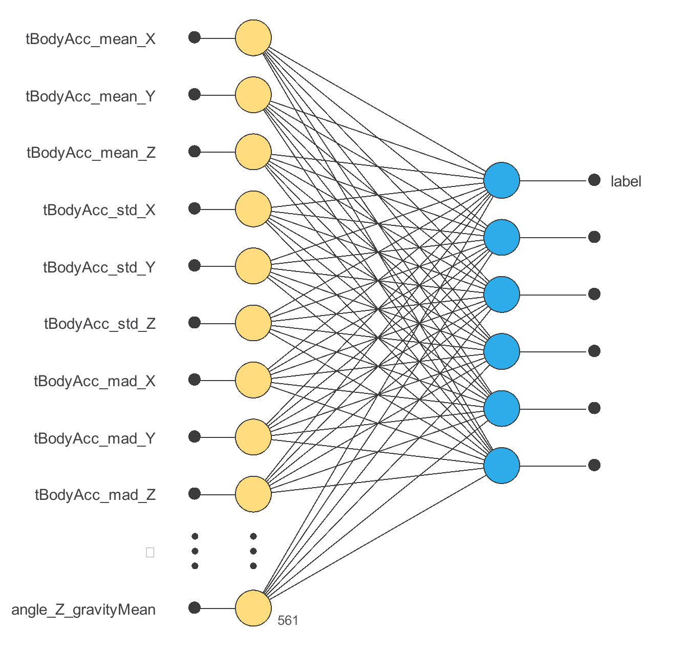
The model has 561 encoded inputs and 6 outputs. No architecture-selection experiment is recorded in this project. The diagram shows the topology used by the saved model.
| Layer | Input shape | Output shape | Activation |
|---|---|---|---|
| Scaling | 561 | 561 | |
| Dense | 561 | 6 | Softmax |
Output values are uncalibrated model scores. Use the output encodings and decision rule documented with this project; do not assume independent sigmoid scores sum to one.
4. Training strategy
The saved training configuration uses QuasiNewton with CrossEntropy.
No separate completed training task is stored in this report. The optimizer configuration is not evidence that a training run completed; no loss or epoch result is reported here.
5. Model selection and baseline
No model selection experiment is recorded for this version. The validation subset guides fitting where a training report is present; it is distinct from the held-out test rows.
6. Clinical validation
The supplied .nd has no saved testing analysis. Its 2059 testing-role records are a configured subset, not an evaluated result. No accuracy, sensitivity, specificity, precision or ROC AUC is available for this current version.
7. Workflow and reproducibility
Use the same input schema and category order when calculating outputs.
Research workflow: eligible record or image → measurement and schema checks → model score → expert review → confirmatory clinical method where appropriate. No model output should be used as an autonomous diagnosis or treatment instruction.
8. Safety, generalizability and governance
The CSV does not include participant identifiers for a subject-grouped audit. The model’s random row roles do not establish new-participant performance, and the adapted numerical values should be checked against the source preprocessing before reproducing normalized HAR benchmarks. Complete and save the training and evaluation tasks before reporting metrics. No external validation is documented. Physiological-signal specialist and expert review are needed to assess subject transfer.
References
- Human Activity Recognition Using Smartphones. Jorge Reyes-Ortiz; Davide Anguita; Alessandro Ghio; Luca Oneto; Xavier Parra. https://doi.org/10.24432/C54S4K
- Dataset terms: Creative Commons Attribution 4.0 International.