The modeling process is the sequence of steps used to build a mathematical model that represents a system or phenomenon from data, so it can be used to make predictions or decisions.
Neural networks are the most crucial technique for machine learning and artificial intelligence. Indeed, building a model consists of finding a function that causes a loss functional to assume an extreme value.
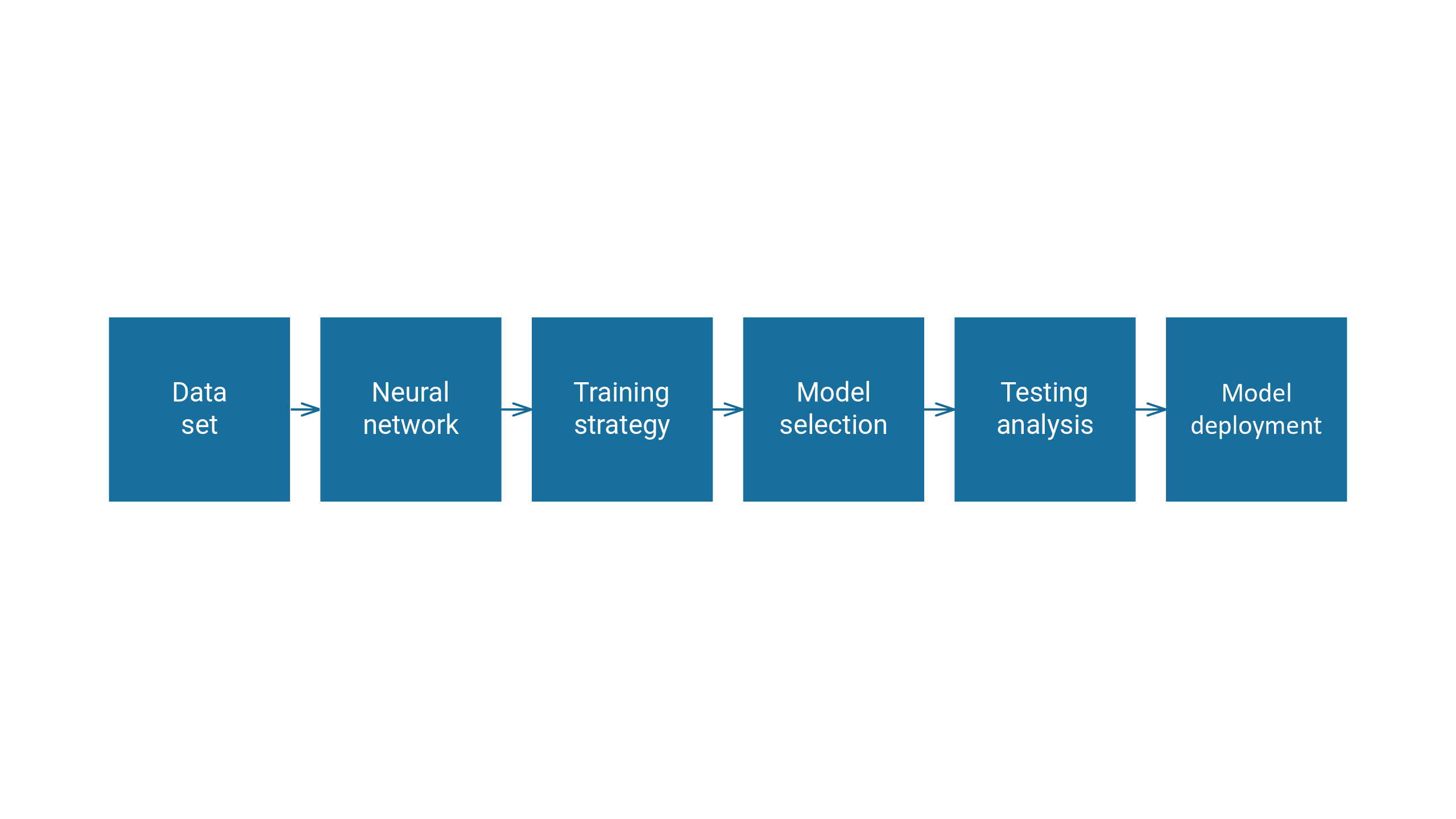
The following figure illustrates a class diagram that represents the concepts involved in the modeling process.
Contents
Next, we introduce these six concepts.
1. Dataset
The data set contains information for creating our model.
The information may include numerical measurements, text, images, and other relevant content.
It is a data collection structured in a table format, consisting of rows and columns.
A dataset comprises a matrix and information about the columns or variables, as well as the rows or samples.
Variables can be used as inputs, targets, or unused.
Samples can be used for training, selection, testing, or unused.
The following is an example of a data set in the automotive sector.
Example: Electric motor data set
An automotive company aims to develop a digital twin of an electric motor utilizing artificial intelligence.
Having robust rotor and stator temperature estimators helps the automotive industry improve the motor’s efficiency by reducing power losses and, ultimately, heat buildup.
The company uses the dataset to build the model.
Then, the dataset comprises various sensor data collected from a permanent magnet synchronous motor (PMSM) deployed on a test bench.
The LEA department of the University of Paderborn collected the testbed measurements.
This data set consists of 107 samples.
See he following table that illustrates the data set.
| ambient temperature | coolant temperature | voltage_d | voltage_q | … | stator_winding |
|---|---|---|---|---|---|
| -0.274 | -1.070 | 0.180 | 1.681 | … | -0.331 |
| -0.274 | -1.070 | -1.243 | 0.483 | … | 0.712 |
| -0.274 | -1.070 | -1.560 | -0.504 | … | 1.519 |
| -0.274 | -1.070 | 0.298 | 0.958 | … | -1.767 |
| -0.274 | -1.070 | -0.963 | 0.642 | … | -0.846 |
| -0.274 | -1.070 | -1.498 | -0.140 | … | -0.947 |
| -0.274 | -1.070 | -1.026 | 0.926 | … | -0.346 |
| … | … | … | … | … | … |
| -0.127 | 1.930 | 0.300 | -1.292 | … | 0.372 |
In this dataset, all variables are numeric.
The input variables are ambient_temperature, coolant_temperature, voltage_d, voltage_q, voltage_module, current_d, current_q and current_module.
On the other hand, target variables are motor_speed, torque, stator_yoke and stator_tooth, stator_winding.
The samples are divided into 60% training samples (65), 20% selection samples (21), and the remaining 20% testing samples (21).
2. Neural network
An artificial neural network, or simply a neural network, can be defined as a biologically inspired computational algorithm consisting of a network architecture composed of artificial neurons.
This structure contains a set of parameters tuned to perform specific tasks.
The neural network represents the model.
Neural networks are organized in layers.
- Approximation models typically contain a scaling layer, a hidden dense layer, an output dense layer, and an unscaling layer.
- Classification models usually contain a scaling layer and an output dense layer.
- Forecasting models typically include a scaling layer, a recurrent layer, a dense layer, and a uscaling layer.
- Other models, such as image classification models, include multiple convolutional and pooling layers, as well as a perceptron or probabilistic layer.
Neural networks have universal approximation properties. This means they can approximate any function in any dimension with a desired degree of accuracy.
The following is an example of a neural network in the automotive sector.
Example: Electric motor neural network
To create its model, the company chooses a neural network.
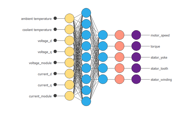
The following figure shows the neural network model.
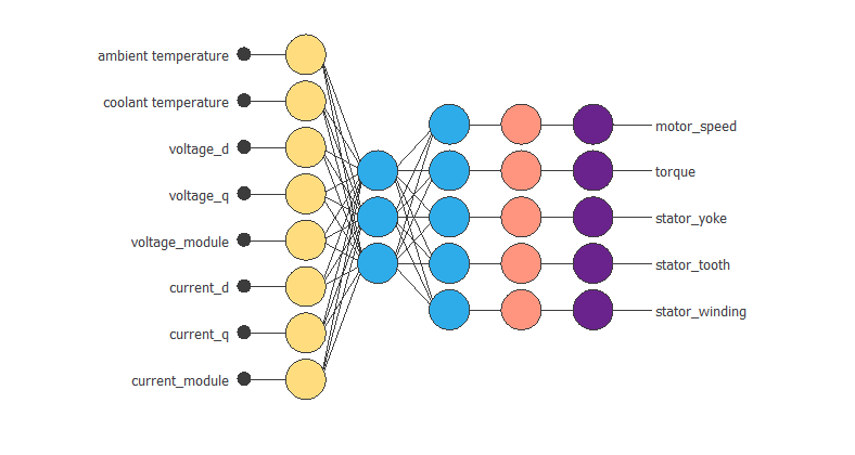
The neural network consists of five layers. The first is a scaling layer with eight neurons; the following are dense layers with three and five neurons, respectively, and the last is a probabilistic layer with five neurons.
As we can see, the inputs to this neural network are ambient_temperature, coolant, voltage_d, voltage_q, current_d, current_q, voltage_module, and current_module.
The outputs from the neural network are motor speed, torque, stator yoke, stator tooth, and stator winding.
3. Training strategy
A training strategy aims to fit the data set to the neural network. It comprises two components: a loss index and an optimization algorithm. The loss index defines the task the neural network must perform and measures the quality of the representation the model is required to learn. Choosing a suitable error term depends on the particular application, and we can state the learning problem as minimizing this loss index.
A loss index is composed of several terms, the most important being the error term and the regularization term. While the error term measures the difference between the outputs of the neural network and the correct predictions, the regularization term controls the model’s complexity to improve generalization.
We can use several types of errors. The most common error functions are Mean Squared Error, Normalised Squared Error, Minkowski Error, Cross-Entropy Error in classification problems, or the Squared Weighted Error in binary classification problems.
The regularization term can be applied to achieve good generalization. Adding a regularisation term to the error term will decrease the values of the biases and the neural network’s weights.
Consequently, the outputs of the neural network will become smoother, thereby reducing the likelihood of overfitting. One of the most used regularisation methods is the norm of the neural network parameters.
The primary purpose of the loss index is to prevent overfitting and enhance regularization.
Among the most commonly used optimisation algorithms are the Quasi-Newton Method, Levenberg-Marquardt, Stochastic Gradient Descent, and Adaptive Moment Estimation.
The following is an example of a training strategy in the automotive sector.
Example: Electric motor training strategy
An automotive company builds a model to improve the efficiency of its engines. For the loss index, it selects the normalized squared error with L2 regularization, the default choice in approximation applications. As the optimization algorithm, it uses the quasi-Newton method. Once this strategy has been set, we can train the neural network. The figure below shows how the training error (blue) and the selection error (orange) decrease with each epoch during the training process.
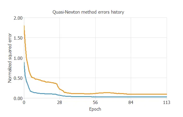
As the chart shows, both errors decrease until they reach a stationary value, which indicates that the algorithm has converged. The most critical result is the final selection error, since it measures the neural network’s ability to generalize to new data. In this case, the final selection and training errors are 0.083 NSE and 0.029 NSE, respectively.
4. Model selection
As we mentioned earlier, the objective of building a model is not to memorize the training subset, but to demonstrate good generalization capacity.
The optimal architecture is the one that shows the best generalization capacity. That is the one for which the selection error is the lowest.
We can analyze which input variables are redundant and can be removed from the neural network, a process known as input selection.
It can be studied to determine the number of neurons for which the neural network shows the best performance, a process known as neuron selection.
When designing the neural network architecture, two common problems can occur: underfitting and overfitting.
Underfitting is the phenomenon that occurs when the model is too simplistic. In this case, the neural network cannot fit either the training data or the selection data.
Overfitting is the opposite effect. It occurs when the neural network is too complex. Consequently, during the training process, the error for the training samples will decrease while the error for the selected samples increases.
In both situations, the result is a model of bad quality.
The following is an example of a model selection in the automotive sector.
Example: Electric motor model selection
To achieve the model’s optimal architecture, the company studies which input variables are redundant and determines the optimal number of neurons for the neural network to exhibit the best performance. This reduces the selection error in its model.
They use the growing neuron algorithm to achieve the optimal number of neurons.
The following figure shows the final neural network model.
Therefore, the number of neurons in the perceptron layer has increased from 3 to 9, and the selection error has changed from 0.083NSE to 0.043NSE.
5. Testing analysis
Once the optimization algorithm has trained the model, we must evaluate its predictive ability on new data that has not been previously seen by the neural network.
We use the test subset, which contains a set of new cases with their corresponding inputs and target variables.
The goal of testing is to compare the responses of the trained neural network with the correct predictions for each sample in the test subset.
We can use the results of this process as a simulation of what would happen in a real-world situation.
One of the simplest methods to study the neural network’s performance is to calculate the error for the testing subset.
If the model has not over-fitted the training or selection instances, the training, selection, and testing errors should be similar.
The most common method for testing regression models is the goodness-of-fit analysis.
In the case of classification, the confusion matrix, binary classification tests, or the ROC curve are commonly used testing methods.
There are also specific methods for testing forecasting models. Some of them are autocorrelations of errors and cross-correlations between input errors.
If we consider the neural network to be of high quality, we can proceed to the deployment phase.
The following is an example of a testing analysis in the automotive sector.
Example: Electric motor testing analysis
Next, the automotive company tests the model to check how well it fits a set of observations. To do this, they calculate its goodness of fit and the coefficient of determination, R². Across the 21 test samples, the goodness-of-fit measures summarize the discrepancy between the observed and the expected values, while the R² coefficient quantifies the proportion of variation in the predicted variable relative to the actual values. A perfect fit, where the results equal the targets, would yield an R² of 1. The figure below illustrates the predicted values versus the actual ones for the output stator_yoke.
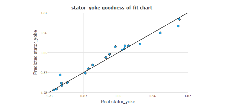
The chart indicates that the predicted values closely align with the actual values.
To give a quality measure, we calculate the coefficient of determination, R2.
| Value | |
|---|---|
| Determination | 0.970 |
Indeed, the R-squared coefficient (R2) is close to 1.
6. Model deployment
Deployment in machine learning refers to applying a model to predict new data.
The deployment of a model consists of making it available to end-users.
There are many ways to deploy a machine learning model.
The form of deployment depends on the requirements.
Sometimes, the end-user wants a report with the results.
On other occasions, they may need a repeatable and continuous learning process.
The following is an example of a model deployment in the automotive sector.
Example: Electric motor model deployment
This mathematical function describes the motor’s operation based on the input data. Below, we write the mathematical expression represented by the neural network.
scaled_ambient temperature = (ambient temperature+0.6031910181)/0.98526299;
scaled_coolant temperature = (coolant temperature+0.3932940066)/1.030290008;
scaled_voltage_d = (voltage_d+0.3587549925)/0.799169004;
scaled_voltage_q = (voltage_q+0.2354030013)/0.9717490077;
scaled_voltage_module = (voltage_module-1.255239964)/0.4234420061;
scaled_current_d = (current_d-0.08343230188)/1.120489955;
scaled_current_q = (current_q-0.2310259938)/0.6012690067;
scaled_current_module = (current_module-1.189710021)/0.4886389971;

perceptron_layer_1_output_0 = tanh( -0.293822 + (scaled_ambient temperature*0.017537) + (scaled_coolant temperature*0.277449) + (scaled_voltage_d*-0.147449) + (scaled_voltage_q*0.0689801) + (scaled_voltage_module*-0.0169951) + (scaled_current_d*-0.267293) + (scaled_current_q*-0.385712) + (scaled_current_module*0.0363538) );
perceptron_layer_1_output_1 = tanh( -0.00602507 + (scaled_ambient temperature*-0.0122427) + (scaled_coolant temperature*-0.447815) + (scaled_voltage_d*-0.036908) + (scaled_voltage_q*0.00900047) + (scaled_voltage_module*-0.0253258) + (scaled_current_d*0.27237) + (scaled_current_q*-0.163464) + (scaled_current_module*-0.115275) );
perceptron_layer_1_output_2 = tanh( 0.224242 + (scaled_ambient temperature*-0.00884039) + (scaled_coolant temperature*-0.210512) + (scaled_voltage_d*-0.0931465) + (scaled_voltage_q*0.0881369) + (scaled_voltage_module*0.0192406) + (scaled_current_d*-0.0520755) + (scaled_current_q*0.185785) + (scaled_current_module*-0.0117133) );

perceptron_layer_2_output_0 = ( 0.141026 + (perceptron_layer_1_output_0*2.54465) + (perceptron_layer_1_output_1*0.551241) + (perceptron_layer_1_output_2*2.39387) );
perceptron_layer_2_output_1 = ( -0.723429 + (perceptron_layer_1_output_0*-1.79491) + (perceptron_layer_1_output_1*-1.76963) + (perceptron_layer_1_output_2*1.484) );
perceptron_layer_2_output_2 = ( 0.231167 + (perceptron_layer_1_output_0*0.653582) + (perceptron_layer_1_output_1*-1.86523) + (perceptron_layer_1_output_2*-0.536217) );
perceptron_layer_2_output_3 = ( 0.155599 + (perceptron_layer_1_output_0*1.09885) + (perceptron_layer_1_output_1*-1.7018) + (perceptron_layer_1_output_2*0.494817) );
perceptron_layer_2_output_4 = ( 0.0824158 + (perceptron_layer_1_output_0*1.09379) + (perceptron_layer_1_output_1*-1.57303) + (perceptron_layer_1_output_2*1.0116) );

unscaling_layer_output_0=perceptron_layer_2_output_0*1.132040024-0.06418219954;
unscaling_layer_output_1=perceptron_layer_2_output_1*0.604493022+0.2313710004;
unscaling_layer_output_2=perceptron_layer_2_output_2*0.9934260249-0.4365360141;
unscaling_layer_output_3=perceptron_layer_2_output_3*1.083299994-0.401120007;
unscaling_layer_output_4=perceptron_layer_2_output_4*1.152959943-0.3688929975;
This mathematical function is the final result of the study. With it, the company can achieve its objective: to improve the efficiency of its car engines.
Tutorial video
You can watch the video tutorial to help you complete this article.
References
- Kaggle Machine Learning Repository. Electric Motor Temperature Data Set.