Introduction
Breast cancer is one of the most common malignancies, and early detection is essential to improve outcomes.
Fine needle aspiration (FNA) biopsies are commonly used, but interpretation can be complex.
Neural networks analyze cellular features from digitized images to assist clinicians.
Using the University of Wisconsin dataset, our model reached an AUC of 0.997 and 98.5% of accuracy, showing the potential of AI to complement expertise, reduce uncertainty, and improve diagnostic decisions.
Healthcare professionals can test this methodology by downloading Neural Designer
Contents
The following index outlines the steps for performing the analysis.
1. Model type
- Problem type: Binary classification (malignant or benign tumor)
- Goal: Model the probability of a malignant tumor based on fine needle aspiration (FNA) test features to support clinical decision-making using artificial intelligence and machine learning.
2. Dataset
Data source
The breast_cancer.csv dataset (683 instances, 10 variables) for a binary classification problem (target: 0 or 1).
Variables
Cell structure
clump_thickness (1–10) – Benign cells form monolayers; malignant cells form multilayers.
cell_size_uniformity (1–10) – Cancer cells vary in size and shape.
cell_shape_uniformity (1–10) – Cancer cells vary in shape and size.
single_epithelial_cell_size (1–10) – Enlarged epithelial cells may be malignant.
bare_nuclei (1–10) – Nuclei without cytoplasm, often in benign tumors.
bland_chromatin (1–10) – Uniform chromatin in benign cells; coarse in cancer cells.
normal_nucleoli (1–10) – Small in normal cells, enlarged in cancer cells.
Cell behaviour
marginal_adhesion (1–10) – Loss of adhesion is a sign of malignancy.
mitoses (1–10) – High values indicate uncontrolled cell division.
- diagnose (0 or 1) – Benign (0) or malignant (1) breast lump.
Instances
The dataset’s instances are split into training (60%), validation (20%), and testing (20%) subsets by default. You can adjust them as needed.
Variables distributions
We can calculate variable distributions; the figure shows a pie chart of malignant (1) versus benign (0) tumors in the dataset.
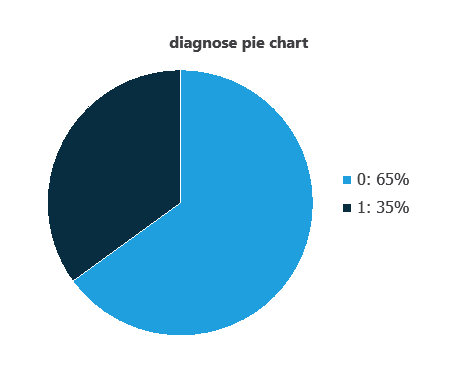
As depicted in the image, malignant tumors represent 35% of the samples, and benign tumors represent approximately 65%.
Input-target correlations
The input-target correlations indicate which factors most influence whether a tumor is malignant or benign and, therefore, are more relevant to our analysis.
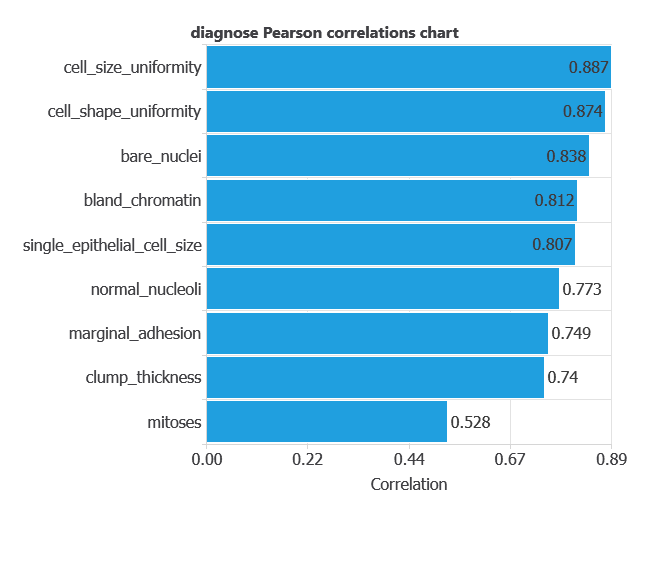
Here, the most correlated variables with malignant tumors are cell size uniformity, cell shape uniformity, and bare nuclei.
3. Neural network
A neural network is an artificial intelligence model inspired by how the human brain processes information. It is organized in layers: the input layer receives the variables, and the output layer provides the probability of belonging to a given class. The network uses historical data to learn patterns distinguishing benign from malignant tumors.
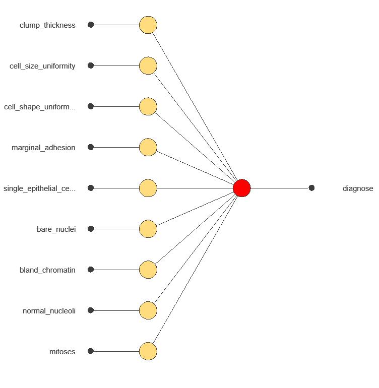
The network uses nine diagnostic variables to output the probability of a malignant tumor, with connections showing each variable’s contribution to the prediction.
4. Training strategy
Training a neural network uses a loss function to measure errors and an optimization algorithm to adjust the model, ensuring it learns from data while avoiding overfitting for good performance on new cases.
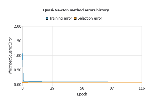
The network was trained to minimize errors while avoiding overfitting, achieving stable performance on new cases (training error 0.054, validation error 0.072).
5. Testing Analysis
The objective of the testing analysis is to validate the generalization performance of the trained neural network.
ROC curve
The ROC curve is a standard tool to evaluate a classification model, showing how well it distinguishes between two classes by comparing predicted results with actual outcomes. A random classifier scores 0.5, while a perfect classifier scores 1.
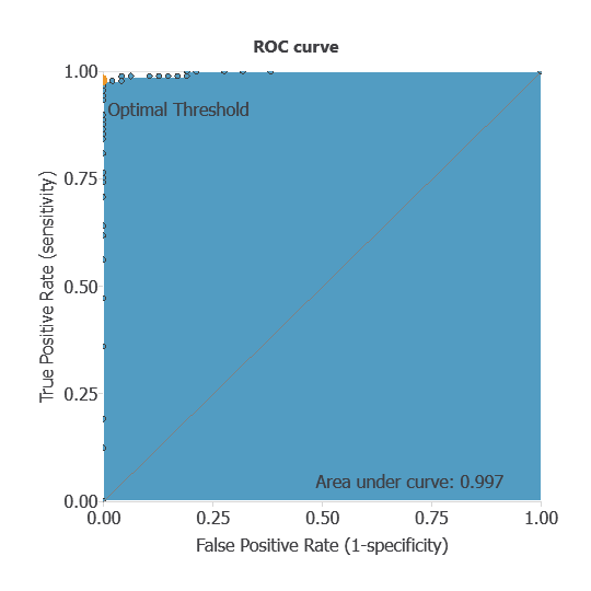
The model achieved an AUC of 0.997, indicating excellent discrimination between benign and malignant tumors.
Confusion matrix
The confusion matrix shows the model’s performance by comparing predicted and actual diagnoses. It includes:
- true positives – tumors correctly identified as malignant
- false positives – benign tumors incorrectly identified as malignant
- false negatives – malignant tumors incorrectly identified as benign
- true negatives – tumors correctly identified as benign
For a decision threshold of 0.5, the confusion matrix was:
| Predicted positive | Predicted negative | |
|---|---|---|
| Real positive | 47 | 0 |
| Real negative | 2 | 87 |
In this case, 98.53% of cases were correctly classified and 1.47% were misclassified.
Binary classification
The performance of this binary classification model is summarized with standard measures:
Accuracy: 98.5% of tumors were correctly classified.
Error rate: 1.5% of cases were misclassified.
Sensitivity: 100% of malignant tumors were correctly identified.
Specificity: 98% of benign tumors were correctly identified.
The model correctly identifies nearly all malignant and benign tumors, confirming its high diagnostic performance.
6. Model deployment
Once validated, the model can be deployed to predict malignancy probabilities for new patients.
In deployment mode, healthcare professionals can use the model as a reliable diagnostic support tool for classifying new patients. The Neural Designer software exports the trained model automatically, making it easy to integrate into clinical practice.
Conclusions
The breast cancer diagnostic model, developed with the University of Wisconsin dataset, showed excellent performance (AUC = 0.997, accuracy = 98.5%) in distinguishing benign from malignant tumors.
Key features—cell size and shape uniformity, and bare nuclei—align with pathological criteria, confirming clinical validity.
With strong generalization capacity, this neural network can serve as a valuable decision-support tool, enhancing early detection, complementing FNA biopsy interpretation, and improving diagnostic accuracy in clinical practice.
References
- We have obtained the data for this problem from the UCI Machine Learning Repository.
- Wolberg, W.H., & Mangasarian, O.L. (1990). Multisurface method of pattern separation for medical diagnosis applied to breast cytology. In Proceedings of the National Academy of Sciences, 87, 9193–9196.
- Zhang, J. (1992). Selecting typical instances in instance-based learning. In Proceedings of the Ninth International Machine Learning Conference (pp. 470–479). Aberdeen, Scotland: Morgan Kaufmann.