
Estimate full-load power output under changing ambient conditions
This neural-network surrogate predicts hourly net electrical power from ambient temperature, exhaust vacuum, atmospheric pressure and relative humidity. It can provide a fast expected-output baseline for performance monitoring, planning and engineering analysis.
Ambient conditions influence gas-turbine air mass flow, condenser performance and the net power available from a combined-cycle plant. A data-driven baseline can estimate the output expected at full load and help engineering teams distinguish normal weather-related variation from performance deviations that deserve investigation.
1. Industrial challenge
This is an approximation problem. The model maps hourly average plant and ambient conditions to energy_output, which represents net electrical power in MW despite the legacy code name.
Potential users include plant managers, performance engineers, operations teams, maintenance and reliability engineers, asset managers, energy planners and industrial data teams.
2. Data set
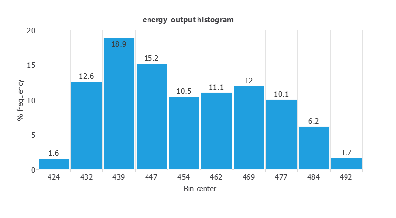
The Combined Cycle Power Plant dataset contains 9,568 hourly averages collected over six years (2006–2011) while the plant operated at full load. Sensor measurements were averaged from higher-frequency readings. The local CSV has no missing values.
| Variable | Engineering meaning | Role | Range |
|---|---|---|---|
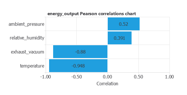
temperature | Ambient temperature (°C) | Input | 1.81 to 37.11 |
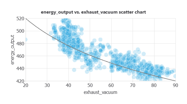
exhaust_vacuum | Steam-turbine exhaust vacuum (cm Hg) | Input | 25.36 to 81.56 |
ambient_pressure | Ambient pressure (mbar) | Input | 992.89 to 1,033.30 |
relative_humidity | Relative humidity (%) | Input | 25.56 to 100.16 |
energy_output | Net hourly electrical power output (MW) | Target | 420.26 to 495.76 |
The project assigns 5,742 rows to training, 1,913 to selection and 1,913 to testing.
3. Model
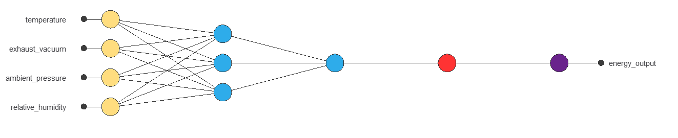
The exported model standardizes the four inputs, processes them with three tanh neurons and returns one linear output that is unscaled to MW. The compact 4–3–1 architecture contains 19 trainable parameters and applies no output bounding.
4. Training strategy
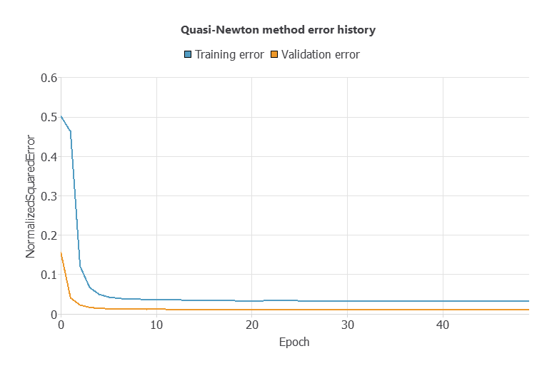
The network minimizes normalized squared error with L2 regularization (weight 0.01) and the quasi-Newton method. Training stopped after 50 epochs because the loss improvement fell below the configured threshold. The final recorded training and selection errors are 0.033 NSE and 0.011 NSE.
5. Model selection
The updated project deploys the compact three-neuron hidden layer and does not contain a saved neuron-selection run. Its training, testing graphic, Python export and browser implementation all describe the same 4–3–1 model.
For a production model, complexity should be selected against a chronological holdout and compared with a simple temperature-based baseline and established plant correction curves. A more complex network is useful only if it improves future-period error consistently.
6. Testing analysis
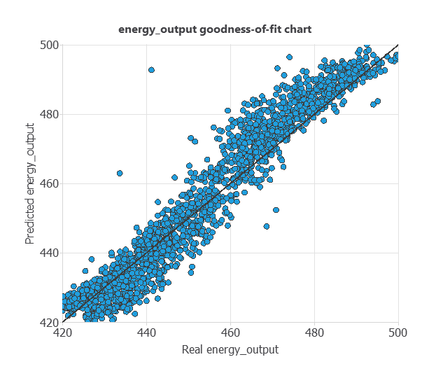
The exported Python model was independently evaluated on the 1,913 rows marked as testing. Neural Designer reports a determination of 0.9377; physical-unit errors show the typical and worst-case discrepancies relevant to plant decisions.
| Testing observations | Determination | Residual R² | MAE | RMSE | 95th-percentile absolute error | Maximum absolute error |
|---|---|---|---|---|---|---|
| 1,913 | 0.9377 | 0.9365 | 3.487 MW | 4.421 MW | 8.469 MW | 37.595 MW |
The model captures most of the full-load variation, but the maximum error is material. Operational use should therefore monitor residuals over time and investigate error by season, operating campaign and maintenance state.
7. Model deployment
A useful deployment compares the model’s expected full-load output with measured output from the historian. Sustained residuals can then trigger engineering review, while short-term dispatch and protection remain in the plant’s certified systems.
Try the full-load power surrogate
Enter hourly average conditions within the dataset ranges. The browser evaluates the exact weights and preprocessing of the exported Python model.
Demonstration surrogate — not a certified control, dispatch or plant-protection system.
Representative hot-ambient scenario
This scenario evaluates a full-load operating point under relatively warm ambient conditions. The four values are passed to the same deployed model used by the browser calculator.
| Input or output | Value |
|---|---|
| Ambient temperature | 29.00 °C |
| Exhaust vacuum | 66.25 cm Hg |
| Ambient pressure | 1,008.00 mbar |
| Relative humidity | 76.00% |
| Predicted net electrical power | 434.03 MW |
The result represents expected full-load power for this combination of conditions. It can support capacity planning or provide a baseline for comparison with measured plant output; it is not a dispatch instruction.
Ambient-temperature derating curve
The directional analysis varies ambient temperature while holding exhaust vacuum at 50.90 cm Hg, ambient pressure at 1,012.60 mbar and relative humidity at 72.43%. At the nominal reference temperature of 20.35 °C, the model predicts 452.74 MW.
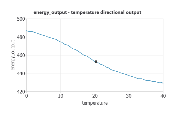
The model shows the expected reduction in available full-load power as ambient temperature rises. The curve must only be interpreted inside the trained temperature range of 1.81 to 37.11 °C; values drawn outside that interval are extrapolations.
Download and reproduce
Tutorial video
8. Scope and limitations
- The data represents one combined-cycle plant operating at full load between 2006 and 2011.
- The released variables are hourly averages and do not model start-up, shutdown, ramps or short transients.
- The model does not include fuel properties, turbine configuration, equipment condition, maintenance events, heat rate, emissions or market constraints.
- The random split and duplicated rows do not prove performance on future years or another plant.
- Inputs must remain within both the numerical ranges and the joint operating combinations represented by the data.
- Production deployment should monitor sensor quality, missing data, residual bias and model drift, with periodic recalibration.
- The surrogate supports engineering analysis; it does not replace OEM correction curves, thermodynamic models, dispatch procedures or certified control and protection systems.
References
- Tüfekci, P., & Kaya, H. (2014). Combined Cycle Power Plant dataset. UCI Machine Learning Repository. DOI: 10.24432/C5002N.
- Tüfekci, P. (2014). Prediction of full load electrical power output of a base load operated combined cycle power plant using machine learning methods. International Journal of Electrical Power & Energy Systems, 60, 126–140.