The original data used in this example is downloaded from the FDA web.

• 1. Introduction
• 2. Materials and methods:
  • 2.1. Data set
  • 2.2. Model development
• 3. Results:

We will use the Neural Designer free version to answer the previous question. You can download a free trial here.

Introduction

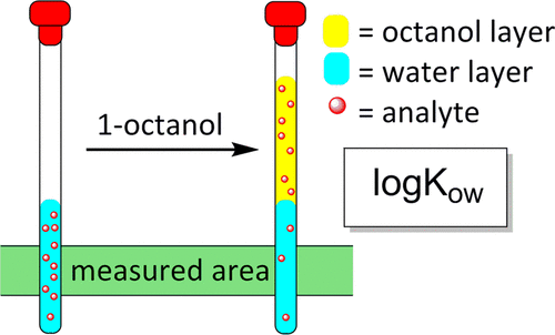
The n-octanol-water partition coefficient, or logK_ow, measures the relationship between a substance’s fat solubility (lipophilicity) and water solubility (hydrophilicity). A substance would be more soluble in fat-like solvents such as n-octanol if the value exceeds one. On the other hand, if this value is less than one, it is more soluble in water.

This value is used, among others, to assess the environmental fate of persistent organic pollutants. Compounds with high coefficients (values greater than 5) tend to accumulate in the organism’s fatty tissue (bioaccumulation).

This value assumes significance in drug research as it offers a reliable estimate of a substance’s distribution within a cell, delineating between membranes (lipophilic) and the cytosol (hydrophilic).

This value is not measurable for all substances, so a good model that allows its prediction will be useful in developing and elaborating drugs for the best treatment of diseases.

Materials and methods

Dataset

This dataset contains physicochemical properties for 16,523 chemical compounds. PubChem, a website detailing chemical compounds and storing their properties, is the source of these properties. All of these properties have been either determined via experimental procedures in the laboratory or via software.

We will download the data from FDA, where the raw files have been processed to tabular format. We also have used the PubChem API to retrieve the physicochemical properties for all the compounds they have records of.

The final merged data has 16523 rows, corresponding to chemical compounds. Each compound has data for 34 physicochemical properties, including the xlogp. This is the value we are going to assess.

Experts calculated this variable using various computational methods and confirmed its accuracy through experimental procedures.

Model development

We will build an approximation model as we try to predict a continuous variable (xlogp).

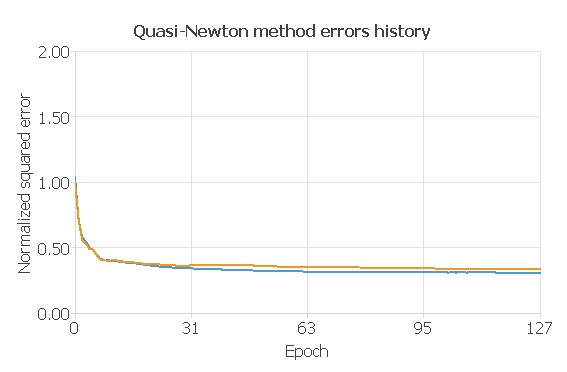
We will use the normalized squared error for the training methodology with a L2 regularization term. As for the optimization algorithm, we will use the Quasi-Newton method.

Also, we will only use variables that we can calculate or infer using the chemical formula of the compound, that is 9 of the 34 properties retrieved from Pubchem:

• MolecularWeigth: mass of a molecule. It is calculated as the sum of the mass of each constituent atom multiplied by the number of atoms of that element in the molecular formula.
• HeavyAtomCount: any atom except hydrogen in a chemical structure.
• Complexity: rough estimate of how complicated a structure is, seen from both the point of view of the elements contained and the displayed structural features, including symmetry. This complexity rating is computed using the Bertz/Hendrickson/Ihlenfeldt formula.
• BondStereoCount: total number of bonds with planar (sp2) stereo [e.g., (E)- or (Z)-configuration].
• DefinedAtomStereoCount: number of atoms with defined planar (sp2) stereo.
• UndefinedAtomStereoCount: number of atoms with undefined planar (sp2) stereo.
• HBondAcceptorCount: the number of hydrogen bond acceptors in the structure.
• HBondDonnorCount: the number of hydrogen bond donors in the structure.

To utilize these properties as input variables, we will employ a network with a scaling layer comprising the same number of neurons as our inputs.

Moreover, the setup involves ten neurons utilizing the hyperbolic tangent as the activation function for the perceptron layer. Additionally, there is an extra perceptron layer employing a linear activation function. Furthermore, we have incorporated unscaling and bounding layers, each with one neuron.

This number of neurons is to obtain better model regularization.

Finally, our probabilistic layer with one neuron gives us the value for the xlogp assessed.

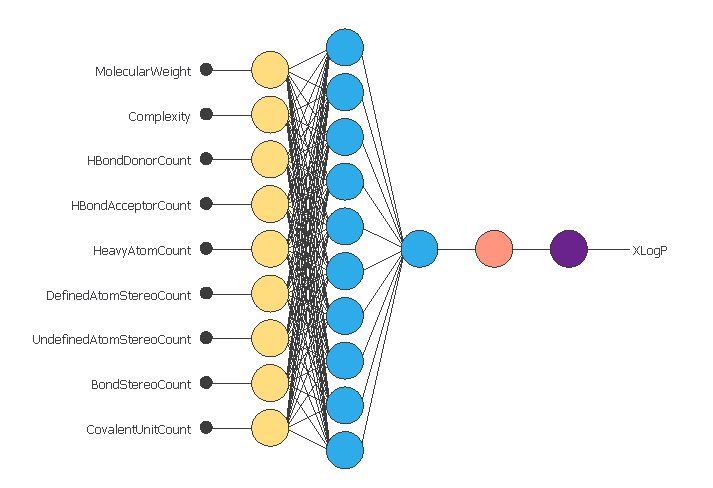
In the previous image, we can see the architecture of the model we will train in the next steps, with all the layers described previously.

Results

We have built a model for predicting the xlogp of chemical compounds. This model gives us the estimated value of this coefficient for a compound.

For our trained model, the training error is 0.308775, and the selection error is 0.337858.

Next, we will use the goodness of fit of our model to describe how well it fits a set of observations. The value we wil be looking at will be the R², which describes how well our model explains the variability of the data. The larger this value, the better our model explains the variability in the data.

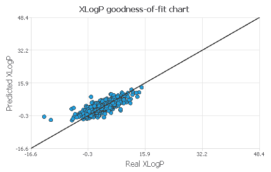
In the previous image, we can see how well we can predict our data, for the ideal case, all the points should be inside the black line. This means that the predicted value is equal to the real value. We have some variance, but more or less, our datapoints are all aggregated near the line. Our model has an R² of 0.64, which means we can explain 64% of the variability in the data.

With this, we can conclude that we have generated a model that works properly to calculate the xlogp of a compound.

References

• Image adapted from: ACS Omega 2017, 2, 9, 6244-6249 September 28, 2017

Related posts