Develop an e-nose to detect alcohols using machine learning

1. Application type

This is a classification project since the variable to be predicted is categorical (1-Octanol, 1-Propanol, 2-Butanol, 2-Propanol, 1-Isobutanol).

2. Data set

The first step is to prepare the dataset, which serves as the source of information for the classification problem.

For that, we need to configure the following concepts:

• Data source.
• Variables.
• Instances.

Data source

The data source is the file QCMalcoholsensor.csv. It contains the data for this example in comma-separated values (CSV) format.

The number of columns is 6, and the number of rows is 26.

Variables

The variables are:

Input variables

Each variable corresponds to the QCM sensor’s resonance frequency when exposed to a specific air–alcohol concentration ratio:

• freq_1 – Frequency at concentration 1 (Air: 0.799 mL, Alcohol: 0.201 mL).
• freq_2 – Frequency at concentration 2 (Air: 0.700 mL, Alcohol: 0.300 mL).
• freq_3 – Frequency at concentration 3 (Air: 0.600 mL, Alcohol: 0.400 mL).
• freq_4 – Frequency at concentration 4 (Air: 0.501 mL, Alcohol: 0.499 mL).
• freq_5 – Frequency at concentration 5 (Air: 0.400 mL, Alcohol: 0.600 mL).

These values capture how the sensor’s oscillation shifts under different mixture concentrations, which is the signal used for classification.

Target variable

• class – The alcohol type detected by the sensor. Possible values are:

• 1-Octanol
• 1-Propanol
• 2-Butanol
• 2-Propanol
• 1-Isobutanol

For machine learning, this categorical variable is typically one-hot encoded as follows:

• 1-Octanol: 1 0 0 0 0.
• 1-Propanol: 0 1 0 0 0.
• 2-Butanol: 0 0 1 0 0.
• 2-Propanol: 0 0 0 1 0.
• 1-Isobutanol: 0 0 0 0 1.

Instances

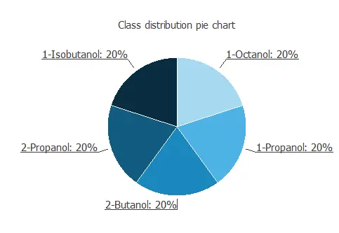
The instances are randomly divided into training, selection, and testing subsets.

They represent 60% (15), 0% (0), and 20% (25) of the original instances, respectively.

Distributions

We can calculate the distributions of all variables. The following figure is a pie chart of the types of alcohol.

As we can see, the target is well-distributed, with the same number for each of the five different alcohol types.

Input-target correlations

Finally, the input-target correlations might indicate to us what factors most influence.

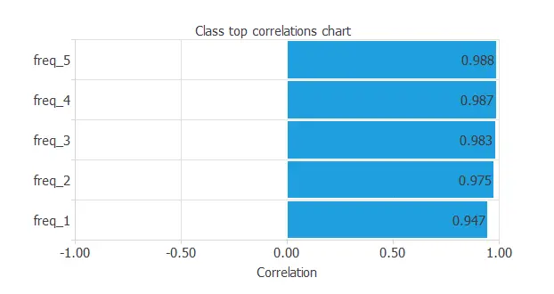
We observe a strong correlation among the variables.

3. Neural network

The second step is to choose a neural network. In classification problems, one typically composes:

• A scaling layer.
• Two perceptron layers.
• A probabilistic layer.

Scaling layer

The scaling layer contains the statistics on the inputs calculated from the data file and the method for scaling the input variables.

Here, we have set the minimum and maximum methods. Nevertheless, the mean and standard deviation method would produce very similar results.

In our case, there is no perceptron layer.

This is because we have little data, so we simplified the program.

The probabilistic layer allows the outputs to be interpreted as probabilities. In this regard, all outputs are between 0 and 1, and their sum is 1.

The softmax probabilistic method is used here.

The neural network has five outputs since the target variable contains 5 classes (1-Octanol, 1-Propanol, 2-Butanol, 2-Propanol, 1-Isobutanol).

4. Training strategy

The fourth step is to establish the training strategy, which comprises:

• Loss index.
• Optimization algorithm.

The loss index chosen for this application is the normalized squared error with L2 regularization.

The error term trains the neural network using the training instances of the dataset.

The regularization term makes the model more stable and improves generalization.

The optimization algorithm searches for the neural network parameters that minimize the loss index. The quasi-Newton method is chosen here.

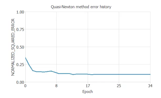
The following chart illustrates how training and selection errors decrease over the course of training epochs.

The final value is the training error, which is 0.109 NSE. The selection error is not visible because we divided the instances into training and testing subsets.

5. Model selection

The objective of model selection is to find the network architecture with the best generalization properties, which minimizes the error on the selected instances of the data set.

Order selection algorithms train several network architectures with different numbers of neurons and select the one with the smallest selection error.

The incremental order method starts with a few neurons and increases the complexity at each iteration.

6. Testing analysis

The purpose of the testing analysis is to validate the model’s generalization performance.

Here, we compare the neural network outputs to the corresponding targets in the test instances of the dataset.

In the confusion matrix, the rows represent the targets (or real values), and the columns represent the corresponding outputs (or predictive values).

The diagonal cells indicate the correctly classified cases, while the off-diagonal cells indicate the misclassified cases.

As we can see, the model correctly predicts all 10 instances (100%), resulting in no misclassified cases.

This shows that our predictive model has excellent classification accuracy.

7. Model deployment

The neural network is now ready to predict outputs for inputs it has never seen.

This process is called model deployment. To classify a given alcohol, we calculate the neural network outputs from the frequencies corresponding to the different types of concentration.

For instance:

• Freq_1: -54.764 Hz.
• Freq_2: -90.826 Hz.
• Freq_3: -132.372 Hz.
• Freq_4: -173.337 Hz.
• Freq_5: -220.833 Hz.

• Probability of 1-Octanol: 1.5 %.
• Probability of 1-Propanol: 9.6 %.
• Probability of 2-Butanol: 1.3 %.
• Probability of 2-Propanol: 24.2 %.
• Probability of 1-Isobutanol: 63.4 %.

In this particular case, our e-nose would classify the alcohol as 1-Isobutanol because it has the highest probability.

Conclusions

We have developed an e-nose algorithm that can be implemented in sensors, like QCM sensors, to detect the corresponding type of alcohol.

References

• UCI Machine Learning Repository. QCM12 Data Set.
• M. Fatih Adak, Peter Lieberzeit, Purim Jarujamrus, Nejat Yumusak, Classification of alcohols obtained by QCM sensors with different characteristics using ABC-based neural network, Engineering Science and Technology, an International Journal, 2019, ISSN 2215-0986.Web Link.

Related posts