This example aims to use machine learning to predict steel properties only by knowing the elements’ concentration percentage and the temperature.

Steel can be alloyed with copper, silicon, or molybdenum to improve or change certain qualities. At the same time, there are no precise theoretical methods to predict mechanical properties because testing each material with different compositions is a tedious process.

1. Application type

The variables to be predicted are continuous. Therefore, this is an approximation project.

The primary goal is to model those properties as a function of the percentages of different materials alloyed and the temperature.

2. Data set

The first step is to prepare the data set, which is the primary source of information. It is composed of:

• Data source.
• Variables.
• Instances.

Data source

The data file LowAlloySteels.csv contains 20 columns and 915 all variables are continuous.

Variables

The variables of the problem are:

• Alloy_code: An identificator for each alloy
• C: Concentration percentage of Carbon
• Si: Concentration percentage of Silicon
• Mn: Concentration percentage of Manganese
• P: Concentration percentage of Phosphorus
• S: Concentration percentage of Sulfur
• Ni: Concentration percentage of Nickel
• Cr: Concentration percentage of Chromium
• Mo: Concentration percentage of Molybdenum
• Cu: Concentration percentage of Copper
• V: Concentration percentage of Vanadium
• Al: Concentration percentage of Aluminum
• N: Concentration percentage of Nitrogen
• Ceq: Concentration percentage of Carbon equivalent
• Nb+Ta: Concentration percentage of Niobinium+Tantalum is constant, so we set it as Unused
• Temperature_C: in degrees Celsius
• 0.2_Proof Strees: Amount of stress resulting in a plastic strain of 0.2%. Measured in MPa
• Tensile_Strenght: Maximum stress that a material can bear before breaking where it can be stretched or pulled. Measured in MPa
• Elongation: Measure deformation before a material breaks when subjected to a tensile load. As a percentage.
• Reduction_in_Area: As a percentage

Our target variables will be the last four 0.2% Proof Stress, Tensile Strenght, Elongation, and Reduction in Area.

In this case, we focus on Elongation, so we select as Unused the other variables. The process for the other properties it’s the same.

Instances

This data set contains 915 instances. From these, 549 instances are used for training (60%), 183 for generalization (20%), and 183 for testing (20%).

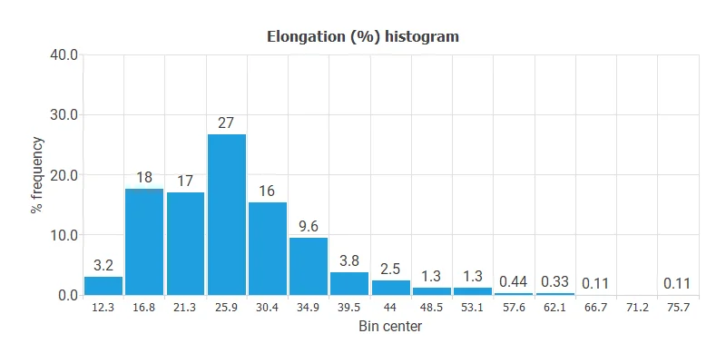
Variables distributions

Calculating the data distributions helps us detect anomalies and correctness. The following chart shows the histogram for the Elongation.

Inputs-targets correlations

It also helps to look for dependencies between input and target variables. To do that, we can plot an inputs-targets correlations chart. This example is the Elongation correlation chart.

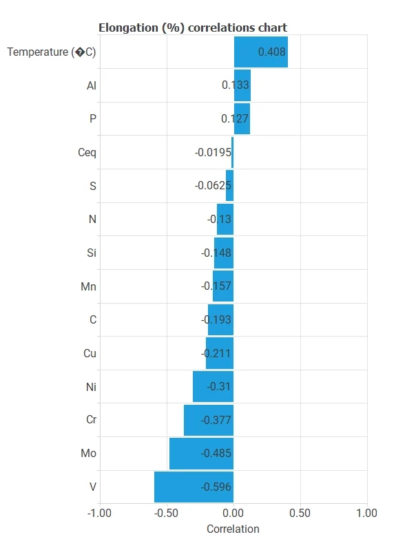
For example, we can see that the Vanadium percentage is the most correlated variable with Elongation.

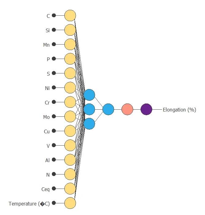
3. Neural network

The next step is to build a neural network representing the approximation function. For approximation problems it is usually composed by:

• A scaling layer.
• Two perceptron layers.
• A probabilistic layer.

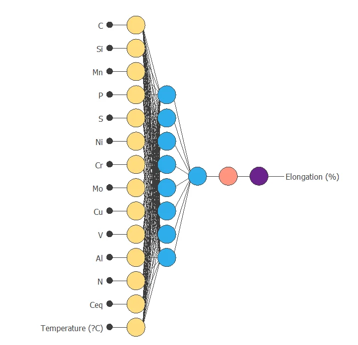
The neural network has 14 (Temperature and percentages of distinct metals alloyed ) inputs and 1 output.

The scaling layer contains the statistics on the inputs. We use the automatic setting for this layer to accommodate the best scaling technique for our data.

We use 2 perceptron layers here:

• The first perceptron layer has 14 inputs, 3 neurons, and a hyperbolic tangent activation function
• The second perceptron layer has 3 inputs, 1 neuron, and a linear activation function

The unscaling layer contains the statistics of the output. We use the automatic method as before.

The following figure shows the neural network structure that has been set for this data set.

4. Training strategy

The fourth step is to select an appropriate training strategy defining what the neural network will learn.

• A loss index.
• An optimization algorithm.

The loss index. defines the quality of the learning. It is composed of an error term and a regularization term.

The error term chosen is the normalized squared error. It divides the squared error between the neural network outputs and the data set’s targets by its normalization coefficient.
If it takes a value of 1 then the neural network predicts the data “in the mean”, while a value of zero means a perfect data prediction. This error term does not have any parameters to set.

The regularization term is L2 regularization. It is applied to control the neural network’s complexity by reducing the parameters’ value.

The optimization algorithm is in charge of searching for the neural network that minimizes the loss index.
Here we choose the Levenberg-Marquardt as the optimization algorithm.

The following chart shows how training and selection errors decrease with the epochs during training.

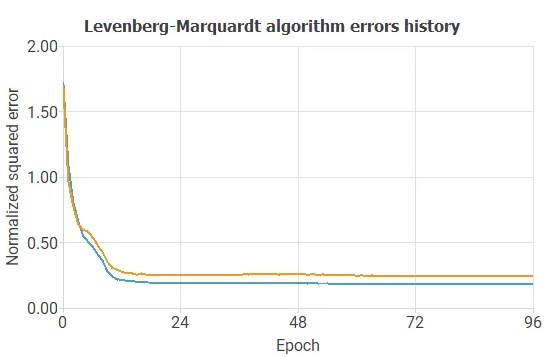
The final values are training error = 0.1821 NSE and selection error = 0.2455 NSE, respectively.

5. Model selection

To improve the selection error, 0.2455 NSE, and the predictions made by the model, we can perform Model Selection algorithms on the structure. The best selection error is achieved by using a model whose complexity is optimal to produce adequate data fit. We use order selection algorithms that find the optimal number of perceptrons in the neural network.

For example, we have the incremental order algorithm. The blue line represents the training error as a function of the number of neurons, and the orange line plots the final selection error as a function of the number of neurons.

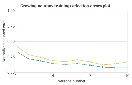
As a result, we obtained a final selection error of 0.1236 NSE with 8 neurons. The following figure shows the optimal network architecture for this case.

6. Testing analysis

Now, we perform various tests to validate our model and see how good the predictions could be. In this case, we perform a linear regression analysis between the predicted and the real values. In the following figure, we can see the relation.

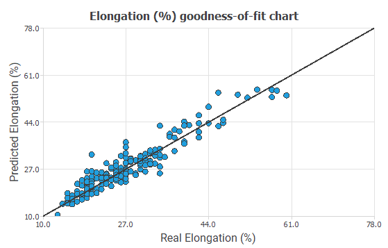
The correlation value is R2=0.8861, which is close to 1.

7. Model deployment

Now we can use the model for estimations on the elongation fixing of some variables or calculate a new estimation with the model.

For example, you can minimize the Elongation, maintaining the proportion of carbon greater than 0.2.

The next table resumes the conditions for this problem.

And the results of our model are :

• C: 0.25%
• Si: 0.412%
• Mn: 0.65%
• P: 0.012%
• S: 0.009%
• Ni: 0.096%
• Cr: 0.44%
• Mo: 0.3958%
• Cu: 0.19%
• V: 0.106%
• Al: 0.37%
• N: 0.004%
• Ceq: 0.1377%
• Temperature: 149.725 ºC
• Elongation: 10.4633%

We can see how the outputs vary when all the inputs are fixed except one with Directional outputs where we can see how the Elongation changes when the temperature increases.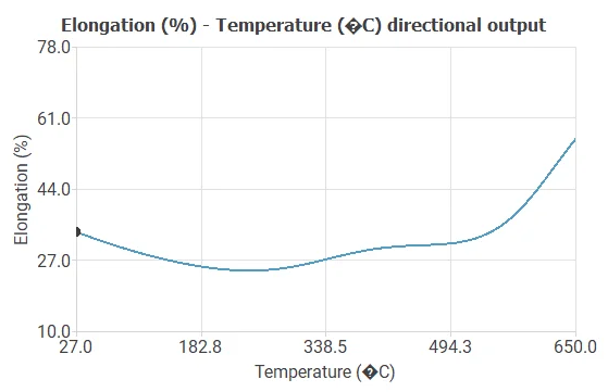

References

• Kaggle open repository: Mechanical properties of low alloy steels.

Related posts