Types and uses of variables in machine learning

1. Definition
2. Variable types
3. Variable uses
4. Conclusions
5. Video tutorial
6. References

1. Definition

A variable can be anything that can be measured or counted, such as a number, trait, or personality trait.

It’s an element that defines something: a person, place, object, or idea.

Moreover, the value of the variable may vary from one sample to another.

For example, variables can represent many different things: physical measurements (temperature, speed, etc.), personal characteristics (gender, age, etc.), marketing dimensions (periodicity, frequency, etc.), pixel values, etc.

In machine learning, the variables are the columns of the data matrix.

A variable is a vector $v in {R}^{p}$, where $p$ is the number of samples in the dataset. In this regard, the data matrix contains $q$ variables,

$begin{eqnarray}
v_{i} := column_{i}(d), quad i=1,ldots,q.
end{eqnarray}$

We can categorize variables according to the type of data or their use in the model.

2. Variable types

We can classify the different types of machine learning variables as numeric, ordinal, binary, categorical, date-time, or id.

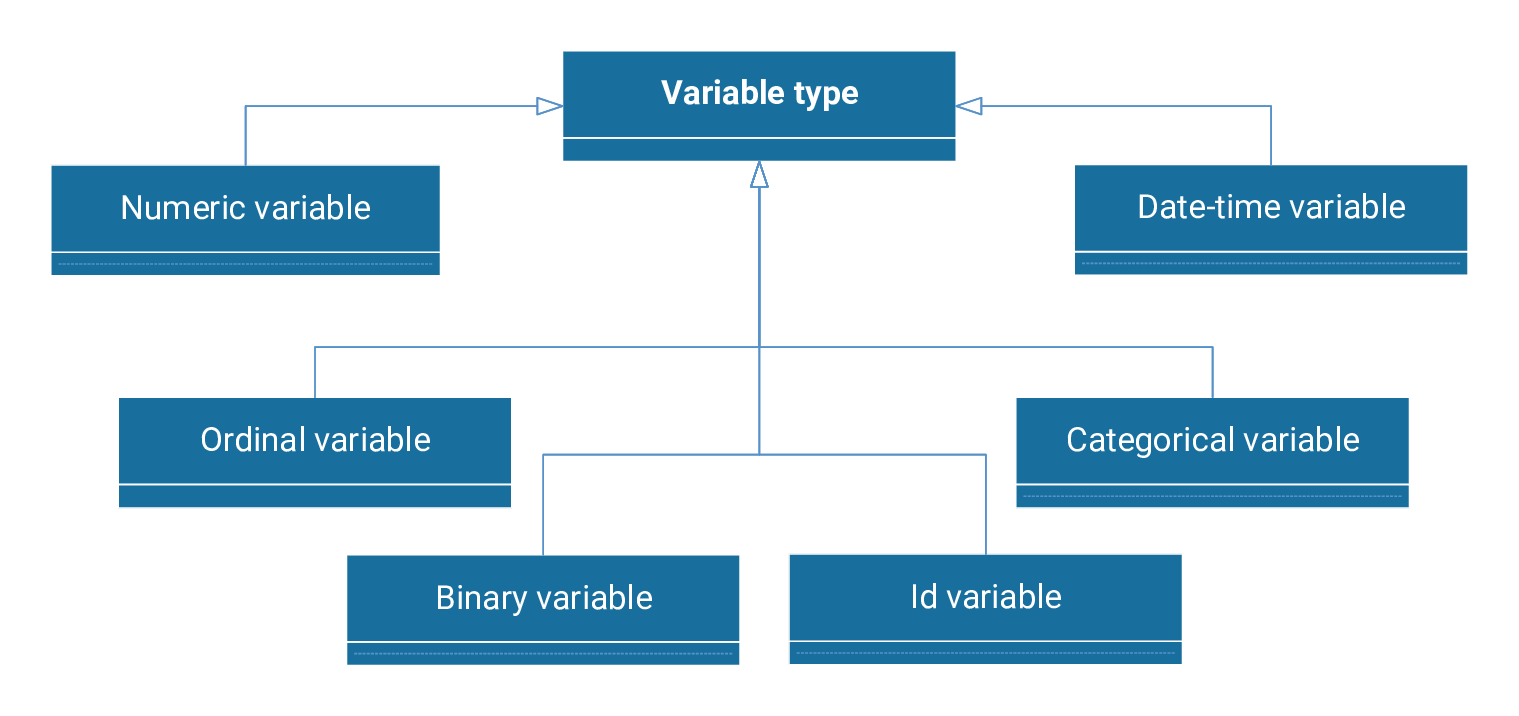
Below, we describe each of these six types of variables.

Numeric variables

Numeric variables have values that describe a measurable quantity as a number, like ‘how many’ or ‘how much.’

They are typically obtained by measuring (i.e., continuous) or counting (i.e., discrete).

For that, we can describe numeric variables as either continuous or discrete.

Since they are actual values, we do not need to treat numeric variables before including them in the data matrix.

Ordinal variables

Ordinal variables exhibit a specific order, unlike categorical variables.

For instance, education levels (such as elementary school, high school, graduate degree) or economic status (low, medium, high) are examples of ordinal data.

Ordinal values can be numerically encoded to facilitate analysis by assigning values in accordance with their order.

For instance, the first value might be denoted as $1$, the second as $2$, the third as $3$, and so forth.

Binary variables

Binary variables have two classes and hold particular significance in data analysis. Typically, they signify the absence or presence of a specific categorical effect that could influence the outcome. For example, a patient may be positive or negative for a disease.

Another example is that a customer may or may not have purchased a product. In these cases, we label the positive value $1$ and the negative value $0$.

Categorical variables

Data characterized by a finite set of possible values often falls within the realm of categorical data. In contrast to numerical data, categorical variables lack a definitive order or hierarchy; instead, they aggregate information into distinct and separate categories. For example, marital status is a categorical variable whose values are single, married, and divorced.

Encoding categorical data involves converting it into an integer format, allowing the models to receive and improve their predictions with the converted values.

For the case of categorical variables with two classes, $C_1$, and $C_2$, we can codify one class as $0$ and the other as $1$.
Therefore, the number of resulting variables is just one. In this way, the value for a sample $j$ is

$begin{eqnarray}
boxed{v_{j} = left{ begin{array}{ll}
0 & textrm{$x_{i,j} in C_{1}$,}\
1 & textrm{$x_{i,j} in C_{2}$,}
end{array} quad i=1, ldots,q. right.}
end{eqnarray}$

We must code the data with the one-hot encoding scheme if the categorical variable has more than two classes, $C_{1}, ldots, and C_{m}$.

In this encoding, each category of any categorical variable receives a new variable. It assigns each category a binary number (0 or 1).

The following table illustrates the one-hot encoding.

After one-hot encoding, the number of resulting variables is the number of categories.

In this way, the variables of a sample $i$ are

$begin{eqnarray}
boxed{v_{j} = left{ begin{array}{ll}
0 & textrm{$x_{j,i} notin C_{k}$,}\
1 & textrm{$x_{j,i} in C_{k}$,}
end{array} quad i=1, ldots,q. right.}
end{eqnarray}$

Date-time variables

A date-time variable encodes a calendar date and a clock time. Additionally, it includes the year, month, day, and second information in a single string. Consequently, human-readable date/time variables are converted to Unix timestamp variables.

Unix timestamps, which track time as the total number of seconds running, serve as an efficient representation. However, it’s important to note that these variables are not included in the model.

Constant variables

Constant variables are those columns in the data matrix that always have the same value. They should be set as unused since they do not provide any information to the model but increase its complexity.

ID variables

The ID variables identify the samples. These variables are not part of the model.

Example: Bank marketing variable types

To facilitate this goal, a banking institution conducts a customer segmentation study to identify the people most likely to be interested in a specific product or service.

Consequently, the bank creates a model to predict which customers will subscribe to a long-term deposit and which will not.

The variables included in the dataset are the following.

• $age$ is numeric. It takes values such as 18, 45, 72, etc.
• $marital status$ is categorical. It takes values divorced, married, and single.
• $default$ is binary.
• $balance$ is numeric. It takes values between -3313 and 71188.
• $housing$ is binary.
• $loan$ is binary.
• $contact$ is binary.
• $day$ is numeric. It takes the different values of the days of the month, from 1 to 31.
• $month$ is numeric. It takes the different values of the month of the year, from 1 to 12.
• $campaign$ is numeric. It takes values between 1 and 50.
• $last contact$ is numeric. It takes values between 1 and 871.
• $previous contacts$ is numeric. It takes values between 0 and 25.
• $past outcome$ is binary.
• $conversion$ is binary.

3. Variable uses

We now discuss input, target, or unused variables regarding their use in a machine learning model.

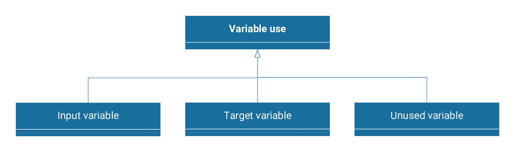
Each of these three uses of variables is described below.

Input variables

Input variables, which serve as the independent variables in the model, play a pivotal role.

Additionally, these variables are referred to as features or attributes within the model’s context.

In our notation, we denote input variables as $x$, and the number of input variables in a data matrix is represented by $n$.

Target variables

Target variables, as the dependent variables in the model, play a crucial role.

Specifically, we denote these target variables as $t$, and the number of target variables in a data matrix is represented by $m$.

In approximation problems, targets manifest as continuous variables, such as power consumption or product quality.

On the other hand, in classification problems, targets are categorical variables (fault, churn, etc.).

In this type of application, targets are also called categories or labels.

Unused variables

Unused variables are neither inputs nor targets. We can set a variable to Unused when it does not provide any information to the model (ID number, address, etc.).

In this regard, we can define a variable using a vector as follows,

$begin{eqnarray}
variables_use = { input lor target lor unused }^{q}.
end{eqnarray}$

The size of this vector is $q$, the number of variables in the dataset.

Note that a variable cannot have two uses at the same time.

For example, we cannot use a variable as input and as output at the same time.

Conclusions

In machine learning, variables are the columns of the data matrix.

Furthermore, we can classify them in different ways: by type or by use.

It is advisable to conduct a study of these variables before developing the model.

Tutorial video

You can watch the video tutorial to help you complete this article.

Related posts