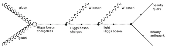
In the early 1960s, particle physicists needed a theory to explain the origin of mass in the universe. In 1964, Peter Higgs theorized the Higgs boson as the fundamental particle responsible for the mass of other elementary particles. That is, a particle able to generate matter as we know it.
Contents
- Application type.
- Data set.
- Neural network.
- Training strategy.
- Model selection.
- Testing analysis.
- Model deployment.
1. Application type
This is a classification project, as the variable to be predicted is binary: either the Higgs boson is present or not.
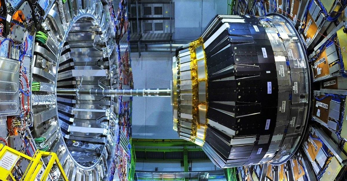
The LHC produces over ten million collisions per hour. However, only a small fraction of these collisions, approximately 300, result in the creation of a Higgs boson. These events are saved to disk, providing approximately one billion events and three petabytes of raw data per year for analysis to obtain evidence of the Higgs boson.
Among these events, we distinguish between those that produce a Higgs boson (signal) and those that are uninteresting (background), which previous experiments have identified. The problem is identifying each event when there is such a large amount of data.
Scientists have collaborated to develop solutions to this problem. On the one hand, we use numerical methods to classify these events, such as a boosted decision tree. On the other hand, we can perform numerical simulations capable of reproducing the signal event where the Higgs boson appears. These simulations provide numerical values for the variables observed with the ATLAS detector.
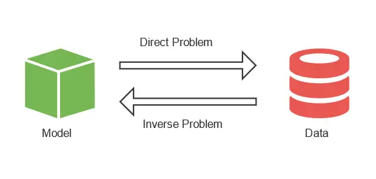
The issue is that we need to classify the raw data obtained from the detector using data from the simulation. This is an inverse problem, where we start from the solution and then obtain the problem’s variables.
In the simulation, we can replicate as many collisions that produce Higgs bosons as we want. This way, we can have similar percentages of both Higgs bosons and uninteresting events. Once we have this data, we create a model to classify the events. It is necessary to utilize machine learning techniques to develop a robust classification model for detecting the Higgs boson. The neural network we obtain provides the probability that a particle is a Higgs boson based on the variables observed by the detector. Finally, we apply this model to the actual data from the LHC. As a result, scientists only have to analyze the particles with a high probability of being a Higgs boson.
2. Data set
The first step is to prepare the dataset, which serves as the source of information for the classification problem. It is composed of:
- Data source.
- Variables.
- Instances.
Data source
The data source is the file Higgs.csv. It contains the data for this example in CSV (comma-separated values) format. The number of columns is 28, and the number of rows is 10012.
The data set consists of 11 million simulated events using the official ATLAS full detector simulator. For this example, we have reduced the instances to around 10000. The proton-proton collisions are simulated based on the knowledge of scientists in particle physics. Next, the resulting particles from the collisions are tracked through a virtual model of the detector.
Each event is described by 28 different features, such as the estimated mass of the Higgs boson candidate or the missing transverse energy.
Variables
The following table shows the variables of the data set for a better understanding of it:
| Variable | Description |
|---|---|
| lepton pT (GeV) | Transverse momentum of the lepton, which can be electrons or tauons. |
| lepton eta (GeV) | Pseudorapidity eta of the lepton. |
| lepton phi (GeV) | Azimuth angle phi of the lepton. |
| Missing energy magnitude (GeV) | Energy that is not detected in a particle detector. |
| Missing energy phi (GeV) | Energy that is not detected in a particle detector. |
| jet 1 pT (GeV) | Transverse momentum of the first jet group. |
| jet 1 eta (GeV) | Pseudorapidity eta of the first jet group. |
| jet 1 phi (GeV) | Azimuth angle phi of the first jet group. |
| jet 1 b-tag (GeV) | Jet consistent with b-quarks. |
| jet 2 pT (GeV) | Transverse momentum of the second jet group. |
| jet 2 eta (GeV) | Pseudorapidity eta of the second jet group. |
| jet 2 phi (GeV) | Azimuth angle phi of the second jet group. |
| jet 2 b-tag (GeV) | Jet consistent with b-quarks. |
| jet 3 pT (GeV) | Transverse momentum of the third jet group. |
| jet 3 eta (GeV) | Pseudorapidity eta of the third jet group. |
| jet 3 phi (GeV) | Azimuth angle phi of the third jet group. |
| jet 3 b-tag (GeV) | Jet consistent with b-quarks. |
| jet 4 pT (GeV) | Transverse momentum of the fourth jet group. |
| jet 4 eta (GeV) | Pseudorapidity eta of the fourth jet group. |
| jet 4 phi (GeV) | Azimuth angle phi of the fourth jet group. |
| jet 4 b-tag (GeV) | Jet consistent with b-quarks. |
| M_jj (GeV) | Transverse momentum of the fourth jet group. |
| M_jjj (GeV) | Pseudorapidity eta of the fourth jet group. |
| M_lv (GeV) | Pseudorapidity eta of the fourth jet group. |
| M_jlv (GeV) | Pseudorapidity eta of the fourth jet group. |
| M_bb (GeV) | Pseudorapidity eta of the fourth jet group. |
| M_wbb (GeV) | Pseudorapidity eta of the fourth jet group. |
| M_wwbb (GeV) | Pseudorapidity eta of the fourth jet group. |
| Event | Signal or Background event. Binary variable. |
Instances
The instances are divided into training, selection, and testing subsets. They represent 60% (6008), 20% (2002), and 20% (2002), respectively, and are split at random.
Variables distributions
We can calculate the distributions of all variables.
The following is a pie chart comparing the Higgs boson to background cases.
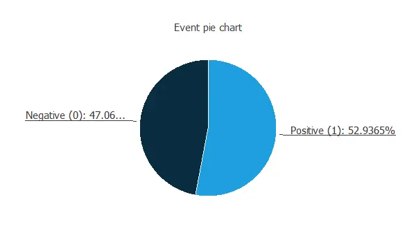
We can see a very similar number of samples for both categories. This is because we have manipulated the data set to improve prediction accuracy. In reality, the background cases represent the majority of the events.
3. Neural network
The second step is to choose a neural network. Classification models usually contain the following layers:
- A scaling layer.
- A hidden dense layer.
- An output dense layer.
Scaling layer
The scaling layer contains the statistics of the inputs calculated from the data file and the method for scaling the input variables. In this case, the minimum-maximum method has been set. Nevertheless, the mean-standard deviation method would produce very similar results.
Hidden dense layer
The number of perceptron layers is one, and it has 4 neurons.
Output dense layer
Finally, we set the binary probabilistic method for the probabilistic layer, as we want the predicted target variable to be binary.
Neural network graph
The following figure is a graph depicting this classification neural network.
Here, the yellow circles represent scaling neurons, the blue circles are the perceptron neurons, and the red circles are the probabilistic neurons.
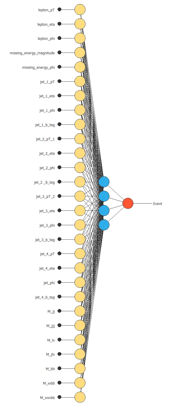
The number of inputs is 28, and the number of outputs is 1.
4. Training strategy
The fourth step is to set the training strategy, which is composed of:
- Loss index.
- Optimization algorithm.
The loss index we choose for this application is the weighted squared error with L2 regularization.
This error term trains the neural network on the training instances of the dataset, while the regularization term stabilizes the model and enhances its generalization.
Additionally, the optimization algorithm searches for the neural network parameters that minimize the loss index. In this context, we choose the quasi-Newton method.
The following chart illustrates how training and selection errors decrease over the course of training epochs.
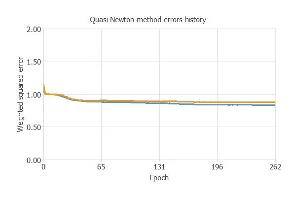
The final values are training error = 0.837 NSE (blue) and selection error = 0.880 NSE (orange).
5. Model selection
The objective of model selection is to find the network architecture with the best generalization properties, which minimizes the error on the selected instances of the data set.
More specifically, we aim to find a neural network with a selection error of less than 0.880 WSE, which is the value we have achieved so far.
Order selection algorithms train several network architectures with different numbers of neurons and select the one with the smallest selection error.
The incremental order method starts with a few neurons and increases the complexity at each iteration.
6. Testing analysis
The last step is to test the generalization performance of the trained neural network.
ROC curve
After training, the testing analysis aims to validate the model’s generalization ability. Specifically, for a classification technique, we need to compare the values predicted by the model to the observed values. Consequently, we can use the ROC curve, the standard testing method for binary classification projects.
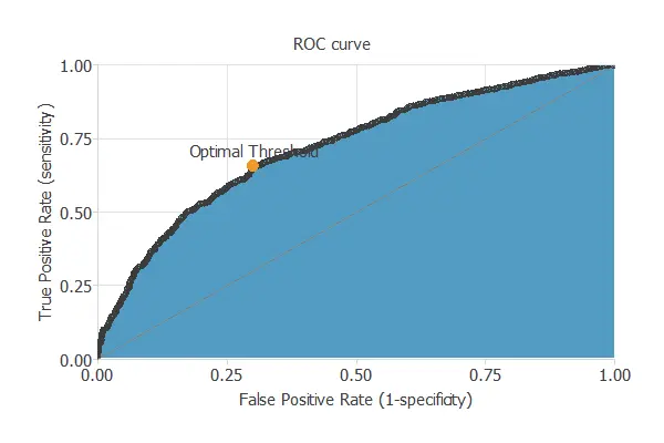
In this case, the area under the ROC curve is 0.720.
Confusion matrix
In the confusion matrix, the rows represent the targets (or real values), and the columns correspond to the outputs (or predictive values).
The diagonal cells show the correctly classified cases, and the off-diagonal cells show the misclassified cases.
| Predicted positive (Higgs Boson) | Predicted negative (background) | |
|---|---|---|
| Real positive (Higgs Boson) | 753 (37.6%) | 307 (15.3%) |
| Real negative (background) | 355 (17.7%) | 587 (29.3%) |
The model correctly predicts 1340 instances (66.9%), while misclassifying 662 (33.1%).
Binary classification metrics
The binary classification tests shown in the following picture provide us with some helpful information about the performance of the model:
- Accuracy (ratio of instances correctly classified): 67%
- Error (ratio of instances misclassified): 33%
- Sensitivity (portion of real positives, which the model predicts as positives): 71%
- Specificity (portion of real negatives that the model predicts as negatives): 62%
7. Model deployment
Once we have tested the model, Neural Designer allows us to obtain its mathematical expression. With it, we can analyze more than four million events per second.
Conclusions
As mentioned, we solved this example with the data science and machine learning platform Neural Designer.
References
- We have obtained the data for this problem from the UCI Machine Learning Repository.
- P. Baldi, P. Sadowski, and D. Whiteson. Searching for Exotic Particles in High-energy Physics with Deep Learning. Nature Communications 5 (July 2, 2014).