Introduction
Obesity prediction with machine learning supports healthcare professionals in delivering personalized recommendations and improving clinical decision-making.
As obesity rates continue to rise in Mexico, Peru, and Colombia, accurate assessment is vital to prevent complications such as diabetes and cardiovascular disease.
Using data on lifestyle, anthropometric measures, and family history, we implemented a neural network model that estimates obesity levels.
Trained with the ObesityDataSet.csv, the model achieved a strong correlation (0.844), showing high potential as a decision-support tool for obesity management.
Healthcare professionals can test this methodology with Neural Designer’s trial version.
Contents
The following index outlines the steps for performing the analysis.
1. Model type
- Problem type: Multiclass classification (seven obesity levels: Insufficient Weight, Normal Weight, Overweight I–II, Obesity I–III)
- Goal: Model the probability of each obesity level based on lifestyle, anthropometric, and family history variables using AI and machine learning to support clinical decision-making.
2. Data set
Data source
The ObesityDataSet.csv dataset contains 2,111 instances and 17 variables for this application.
Variables
The following list summarizes the variables’ information:
Patient information
gender (1=Female, 0=Male) – Sex of the individual.
age (numeric) – Age of the individual in years.
Anthropometric measurements
height (numeric) – Height of the individual in centimeters.
weight (numeric) – Weight of the individual in kilograms.
Family and lifestyle factors
family history with overweight (1=Yes, 0=No) – Indicates if obesity runs in the family.
caloric_food (0=Yes, 1=No) – Frequent consumption of high-caloric food.
vegetables (1, 2, or 3) – Frequency of vegetable consumption.
number_meals (1–4) – Number of main meals per day.
food_between_meals (1=No, 2=Sometimes, 3=Frequently, 4=Always) – Consumption of food between meals.
smoke (0=Yes, 1=No) – Indicates whether the individual smokes.
water (1–3) – Daily water consumption.
calories (0=Yes, 1=No) – Indicates if calorie intake is monitored.
activity (0–3) – Frequency of physical activity.
technology (0–2) – Daily time using technology devices.
alcohol (1=No, 2=Sometimes, 3=Frequently, 4=Always) – Alcohol consumption frequency.
transportation (Automobile, motorbike, bike, public transportation, walking) – Mode of transportation used.
Target variable
obesity_level (categorical) – Classification of obesity level: Insufficient Weight, Normal Weight, Overweight Level I, Overweight Level II, Obesity Type I, Obesity Type II, and Obesity Type III.
Instances
The dataset’s instances are split into training (60%), validation (20%), and testing (20%) subsets by default.
You can adjust them as needed.
Variables distributions
Variable distributions can be calculated; the figure shows the number of samples for each obesity level in the dataset.
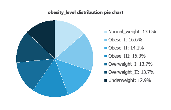
Obesity levels show a semi-normal distribution, ranging from 12.88% (Underweight) to 16.63% (Overweight II).
Input-target correlations
The input-target correlations indicate which variables most influence the obesity level and, therefore, are more relevant to our analysis.
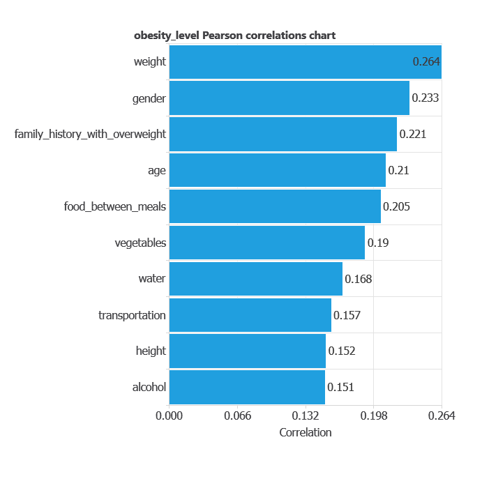
The most correlated variables with obesity level are weight, gender, and family history with overweight.
3. Neural network
A neural network is an artificial intelligence model inspired by how the human brain processes information.
It is organized in layers: the input layer receives the variables, and the output layer provides the probability of belonging to a given class.
Trained with historical data, the network learns to recognize patterns and distinguish between categories, offering objective support for decision-making.
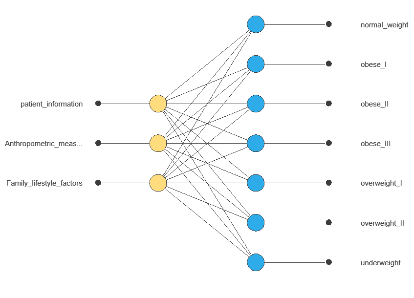
The network uses eighteen individual variables to predict obesity level, with connections showing each variable’s contribution.
4. Training strategy
Training a neural network uses a loss function to measure errors and an optimization algorithm to adjust the model, ensuring it learns from data while avoiding overfitting for good performance on new cases.
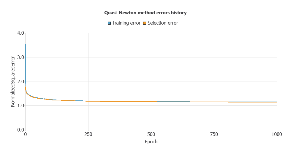
The model was trained for accuracy and stability, with training and selection errors decreasing steadily (1.147 and 1.142 WSE), indicating effective learning and generalization to new instances.
5. Testing analysis
After training, testing analysis compares the neural network outputs with actual target values on unseen data to validate prediction performance and assess readiness for production.
Linear regression analysis
The linear regression analysis illustrates the predicted versus actual obesity levels.
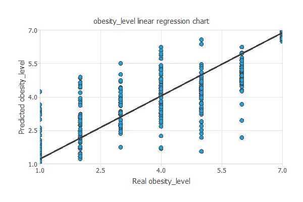
Linear regression of predicted vs. actual obesity levels shows intercept = 0.263, slope = 0.947, and correlation = 0.844, indicating good model performance.
Confusion matrix
The confusion matrix shows the model’s performance by comparing predicted and actual obesity levels. It includes:
True positives: cases correctly classified at the predicted obesity level
False positives: cases incorrectly classified at a higher or lower obesity level
False negatives: cases at a given obesity level incorrectly classified as another
True negatives: cases correctly identified as not belonging to a specific obesity level
| Predicted normal weight | Predicted Obese I | Predicted Obese II | Predicted Obese III | Predicted Overweight I | Predicted Overweight II | Predicted Underweight | |
|---|---|---|---|---|---|---|---|
| Real normal weight | 35 | 3 | 0 | 4 | 1 | 3 | 0 |
| Real Obese I | 6 | 27 | 24 | 9 | 6 | 8 | 3 |
| Real Obese II | 4 | 12 | 32 | 0 | 1 | 3 | 4 |
| Real Obese III | 0 | 0 | 0 | 57 | 0 | 1 | 0 |
| Real Overweight I | 7 | 21 | 2 | 8 | 23 | 4 | 2 |
| Real Overweight II | 9 | 15 | 5 | 5 | 7 | 15 | 0 |
| Real Underweight | 13 | 5 | 0 | 1 | 4 | 0 | 33 |
In this example, 52.61% of cases were correctly classified and 47.39% were misclassified.
6. Model deployment
Once validated, the neural network can be saved for deployment, allowing predictions of obesity level for new individuals based on age, gender, eating habits, and physical activity.
In deployment mode, healthcare professionals can use it as a decision-support tool, with Neural Designer automatically exporting the trained model for easy integration into clinical or research workflows.
Conclusions
The machine learning model achieved high predictive performance (correlation = 0.844) in estimating obesity levels.
The most influential factors—caloric intake, family history of overweight, and age—are consistent with established medical and nutritional evidence, supporting the model’s reliability.
This tool can help healthcare and nutrition professionals assess obesity more accurately, deliver personalized recommendations, and support effective interventions to improve patient outcomes.
References
- We have obtained the data for this problem from the UCI Machine Learning Repository.
- Palechor, F. M., & de la Hoz Manotas, A. (2019). Dataset for estimation of obesity levels based on eating habits and physical condition in individuals from Colombia, Peru and Mexico. Data in Brief, 104344.
- De-La-Hoz-Correa, E., Mendoza Palechor, F., De-La-Hoz-Manotas, A., Morales Ortega, R., & Sanchez Hernandez, A. B. (2019). Obesity level estimation software based on decision trees.