Machine learning tutorial: Neural networks

Dense layer

A dense layer connects every input to every output neuron. Each neuron combines the inputs with trainable weights and a bias, and then applies an activation function. Dense layers learn relationships in tabular, image, and text representations and also produce the final model outputs.

For neuron j, the combination and activation can be written as:

$$z_j=b_j+\sum _{i=1}^n{w}_{ji}{x}_i,y_j=f\left(z_j\right)$$

Neural Designer allows the number of neurons, activation function, and dropout rate to be configured. The main dense activation functions are:

• Linear or identity activation.
• Hyperbolic tangent activation.
• Rectified linear (ReLU) activation.
• Sigmoid activation.
• Softmax activation.

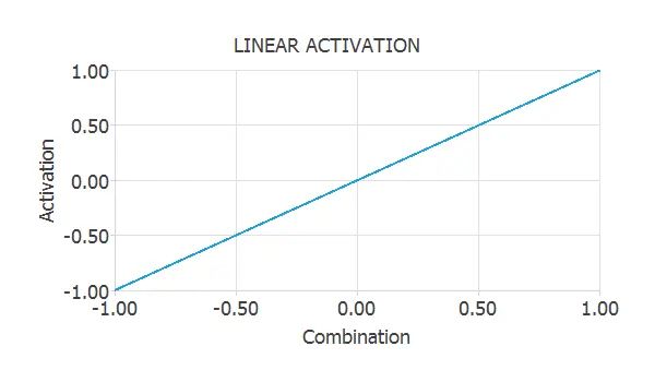
Linear activation function

The linear or identity activation returns the neuron combination unchanged. It is commonly used by output neurons in approximation and forecasting models.

$$f\left(z\right)=z$$

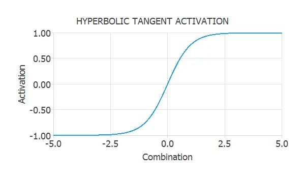
Hyperbolic tangent activation function

The hyperbolic tangent is a sigmoid-shaped function with outputs between -1 and +1. It allows hidden layers to represent positive and negative activations.

$$f\left(z\right)=\tanh \left(z\right)$$

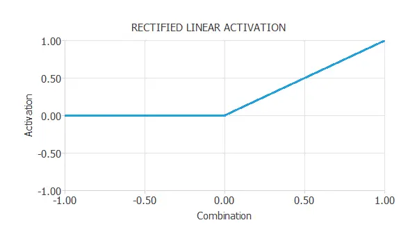
Rectified linear (ReLU) activation function

The rectified linear activation returns zero for negative combinations and the combination itself for positive values. It is widely used in hidden dense and convolutional layers.

$$f\left(z\right)=\max (0,z)$$

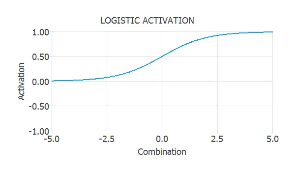
Sigmoid activation function

The sigmoid, also called logistic, activation produces values between 0 and 1. A dense output with one sigmoid neuron represents the positive-class probability in binary classification.

$$f\left(z\right)=\frac{1}{1+e^{-z}}$$

Softmax activation function

Softmax transforms several dense outputs into class probabilities between 0 and 1 whose sum is 1. It is used for multiple classification.

$$y_j=\frac{e^{z_j}}{\sum _{i=1}^n{e}^{z_i}}$$

Convolutional layer

A convolutional layer applies trainable filters, or kernels, across an input image. Each filter detects local spatial patterns such as edges, textures, and shapes and produces an output feature map.

The layer setup defines the number of filters, kernel size, stride, convolution type, and activation function. Neural Designer provides ReLU, linear, hyperbolic tangent, and sigmoid activations for convolutional layers.

For each spatial dimension, the output size is:

$$\text{output size}=\lfloor \frac{\text{input size}+2·\text{padding}-\text{kernel size}}{\text{stride}}\rfloor +1$$

The two available convolution types are:

• Same convolution.
• Valid convolution.

Same convolution

Same convolution adds symmetric padding around the input. With stride 1, it preserves the spatial height and width. Odd kernel sizes such as 3, 5, or 7 keep the padding symmetric.

Valid convolution

Valid convolution does not add padding. The filter is applied only where it completely overlaps the input, so the output feature map is smaller when the kernel is larger than 1.

Convolutional layers are commonly followed by pooling layers. After the spatial features have been extracted, a flatten operation converts the feature maps into a vector for the dense layers.

Pooling layer

A pooling layer summarizes local regions without trainable parameters. For images, it reduces the height and width of feature maps while preserving their channels. The pool size and stride determine the amount of spatial reduction.

The available pooling methods are:

• Maximum pooling.
• Average pooling.

Maximum pooling

Maximum pooling returns the largest value in every pooling region. It preserves the strongest activation and is commonly used after convolutional layers.

Average pooling

Average pooling returns the mean value in every pooling region. It produces a smoother summary of the feature map.

For text models, sequence pooling applies maximum or average pooling across the token dimension. This transforms a sequence of contextual embeddings into one fixed-size vector that can be passed to dense classification layers.

Embedding layer

An embedding layer transforms every token index into a trainable dense vector. Tokens that appear in similar contexts can therefore acquire nearby representations in the embedding space.

The vocabulary size and sequence length come from the text data set, while the embedding dimension determines the size of each token vector. An input sequence with shape sequence length produces an output with shape sequence length × embedding dimension.

Neural Designer scales the token embeddings and adds positional information so that subsequent attention layers can distinguish the order of the tokens. The embedding vectors are learned together with the rest of the network.

Multi-head attention layer

A multi-head attention layer builds contextual token representations by allowing every sequence position to weigh information from the other positions. It projects the embeddings into query, key, and value vectors.

Scaled dot-product attention is calculated as:

$$\text{Attention}(Q,K,V)=\text{softmax}\left(\frac{Q{K}^T}{\sqrt{d_k}}\right)V$$

Several attention heads perform this operation in parallel and learn different relationships between tokens. Their outputs are concatenated and projected back to the embedding dimension. Consequently, the layer preserves the sequence length and embedding dimension.

The number of heads is configurable and must divide the embedding dimension exactly. Multiple multi-head attention layers can be stacked before sequence pooling and dense classification layers.

Long-short-term memory (LSTM) layer

Long-short-term memory (LSTM) layers are a particular recurrent layer widely used in forecasting applications.

The following figure shows an LSTM layer. It receives information as a set of numerical inputs. This information is processed through forget, input, state, and output gates and stored in hidden and cell states. Finally, the layer produces the final outputs.

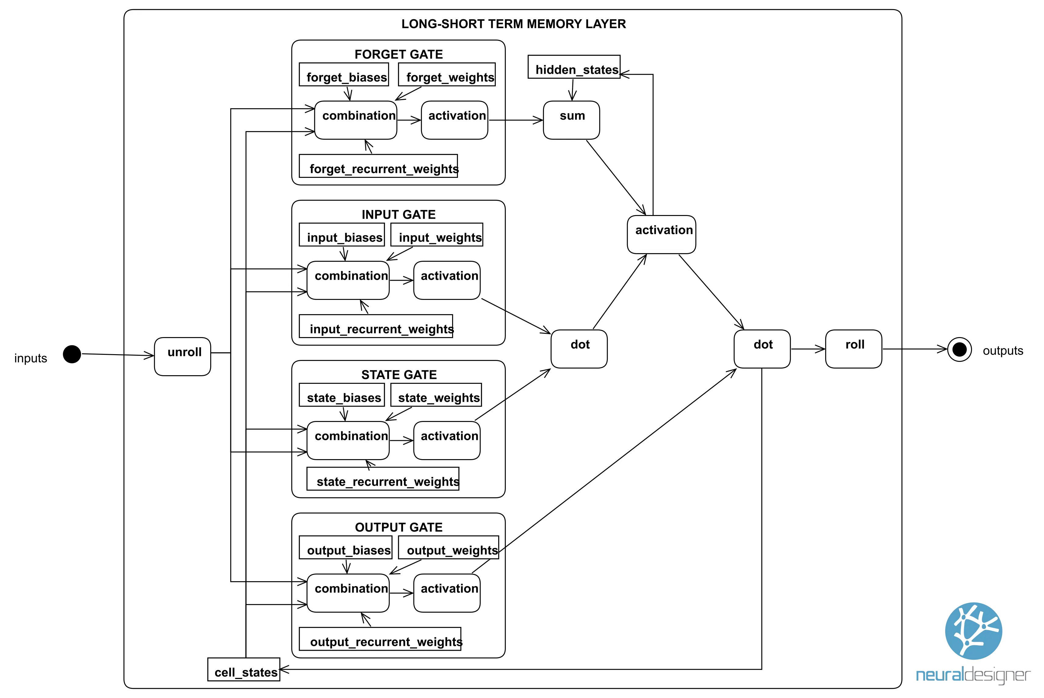
As we can see, long-short-term memory (LSTM) layers are complex and contain many parameters. That structure makes them suitable for learning dependencies from time-series data.

Scaling layer

In practice, scaling the inputs to give them a proper range is always convenient. In the context of neural networks, the scaling layer performs this process.

The scaling layer contains some basic statistics on the inputs. They include the mean, standard deviation, minimum, and maximum values.

Some scaling methods used in practice are the following:

• Minimum and maximum scaling method.
• Mean and standard deviation scaling method.
• Standard deviation scaling method.

Minimum and maximum scaling method

The minimum and maximum methods produce a data set scaled between −1 and 1. This method is usually applied to variables with a uniform distribution.

$$\mathrm{scaled_input} = -1 + \frac{(\mathrm{input} – \mathrm{minimum}) \cdot (1 – (-1))}{\mathrm{maximum} – \mathrm{minimum}}$$

Mean and standard deviation scaling method

The mean and standard deviation method scales the inputs to have a mean of 0 and a standard deviation of 1. This method usually applies to normal (or Gaussian) distribution variables.

$$\mathrm{scaled_input} = \frac{\mathrm{input}}{\mathrm{standard_deviation}}$$

Standard deviation scaling method

The standard deviation scaling method produces inputs with standard deviation 1. This is typically applied to half-normal distributions, variables centered at zero with only positive values.

$$\mathrm{scaled_input} = \frac{\mathrm{input}}{\mathrm{standard_deviation}}$$

All scaling methods are linear and, in general, produce similar results. In all cases, synchronizing the scaling of the inputs in the dataset with the scaling of the inputs in the neural network is necessary. Neural Designer does that without any intervention by the user.

Unscaling layer

The scaled outputs from a neural network are unscaled to produce the original units. In the context of neural networks, the unscaling layer does this.

An unscaling layer contains some basic statistics on the outputs. They include the mean, standard deviation, minimum, and maximum values.

Four unscaling methods are utilized in practice:

• Minimum and maximum unscaling method.
• Mean and standard deviation unscaling method.
• Standard deviation unscaling method.
• Logarithmic unscaling method.

Minimum and maximum unscaling method

The minimum and maximum method unscales variables that have been previously scaled to have minimum -1 and maximum +1, to produce outputs in the original range,

$$\mathrm{unscaled_output} = \mathrm{minimum} + \mathrm{scaled_output} \cdot (\mathrm{maximum}-\mathrm{minimum})$$

Mean and standard deviation unscaling method

The mean and standard deviation method unscales variables that have been previously scaled to have mean 0 and standard deviation 1,

$$\mathrm{unscaled_output} = \mathrm{mean_scaled_output} \cdot \mathrm{standard_deviation}$$

Standard deviation unscaling method

The standard deviation method unscales variables that have been previously scaled to have a standard deviation of 1, to produce outputs in the original range,

$$\mathrm{unscaled_output} = \mathrm{scaled_output} \cdot \mathrm{standard_deviation}$$

Logarithmic unscaling method

The logarithmic method unscales variables that have undergone a logarithmic transformation previously.

$$\mathrm{unscaled_output} = \mathrm{minimum} + 0.5 \cdot \left( e^{\mathrm{scaled_output}} + 1 \right) \cdot (\mathrm{maximum} – \mathrm{minimum})$$

In all cases, synchronizing the scaling of the targets in the dataset with unscaling the outputs in the neural network is necessary. Neural Designer does that without any intervention by the user.

Clamping layer

Some model outputs must remain within a predefined range. For example, a product rating might range from 1 to 5 stars.

The clamping layer applies an individual lower and upper limit to every output. Values inside the interval remain unchanged, while values outside it are set to the closest limit. This final transformation contains no trainable parameters.

$$\text{clamped output}=\min \left(\max \right(\text{output},\text{lower limit}),\text{upper limit})$$

Network architecture

A neural network can be symbolized as a graph, where nodes represent neurons, and edges represent connectivities among neurons. An edge label represents the parameter of the neuron for which the flow goes in.

Most neural networks, even biological neural networks, exhibit a layered structure. Therefore, layers are the basis for determining the architecture of a neural network.

We build a neural network by organizing layers of neurons in a network architecture. The characteristic network architecture in this case is known as the feed-forward architecture. In a feed-forward neural network, we group layers into a sequence so that neurons in any layer connect only to neurons in the next layer.

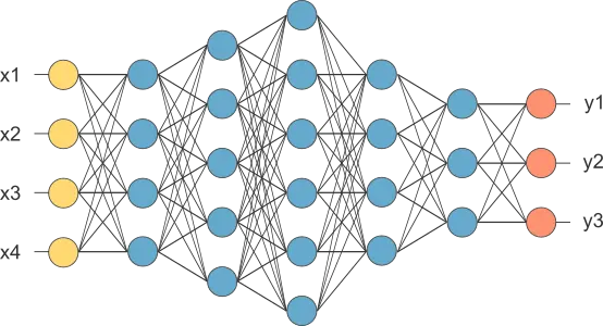
The following figure represents a neural network with four inputs, several layers of different types, and three outputs.

Model parameters

The model parameters involve the parameters of each layer in the network architecture.

You can group all these parameters into a vector (theta), which you can write as:

$$\theta = (\theta_1, \ldots, \theta_d)$$

The number of adaptable parameters, (d), is the sum of parameters in each layer.

As we have seen, a neural network may consist of various types of layers, depending on the requirements of the predictive model.

Next, we describe each application type’s most common neural network configurations.

Approximation neural networks

An approximation model usually contains a scaling layer, one or more dense layers, an unscaling layer, and an optional clamping layer.

Two dense layers are sufficient for many data sets. More complex relationships can require deeper architectures with additional hidden dense layers.

The following figure represents a neural network that estimates the power generated by a combined cycle power plant from meteorological and plant variables.

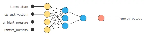
The network has four inputs and one output. It contains a scaling layer, a hidden dense layer with four neurons, an output dense layer with one neuron, and an unscaling layer.

Classification neural networks

A classification model usually contains a scaling layer and one or more dense layers. The final dense layer uses sigmoid activation for binary classification or softmax activation for multiple classification.

Two dense layers are sufficient for many classification data sets, although deeper architectures can learn more complex decision boundaries.

The following figure represents a binary classification model for diagnosing breast cancer from fine-needle aspirates.

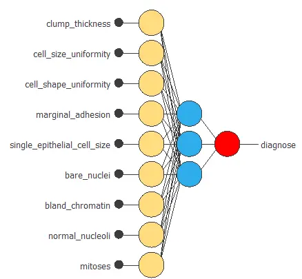
The network has nine inputs and one output. It contains a scaling layer, a hidden dense layer with three neurons, and an output dense layer with one sigmoid neuron.

Forecasting neural networks

A forecasting model can contain a scaling layer, a long short-term memory layer, one or more dense layers, an unscaling layer, and an optional clamping layer.

The following figure represents a one-day-ahead forecasting model for urban NO2 levels.

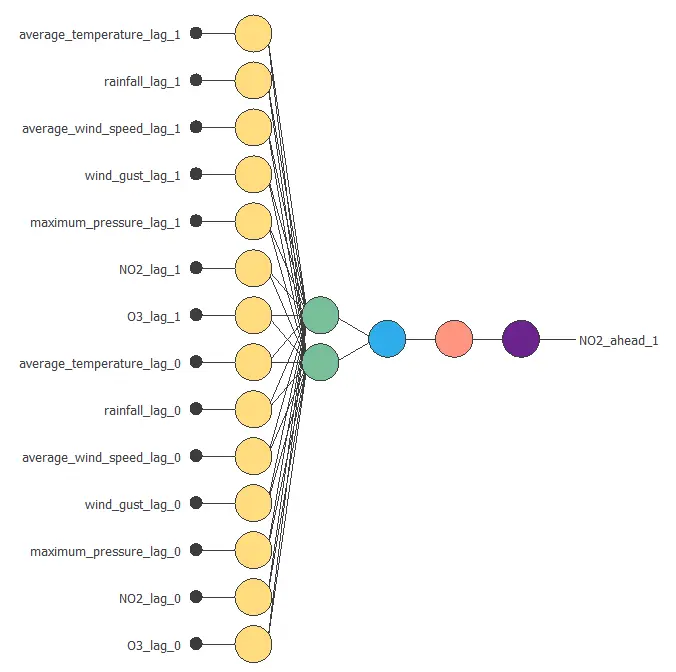
The network has 14 inputs and one output. It contains a scaling layer, an LSTM layer, an output dense layer, an unscaling layer, and a clamping layer.

The inputs contain lagged variables, and the outputs contain the variables for the required forecasting horizon.

Auto-associative neural networks

An auto-associative neural network learns to reproduce its inputs at the outputs. It normally contains a scaling layer, an encoder made of dense layers, a low-dimensional bottleneck, a symmetric decoder, and an unscaling layer.

The encoder compresses the most relevant information into the bottleneck representation. The decoder reconstructs the original variables from that representation.

Reconstruction errors and distances in the bottleneck space can be used to identify unusual samples and detect anomalies.

Convolutional neural networks

A convolutional neural network for image classification starts with image scaling and then stacks convolutional layers and pooling layers.

The convolutional blocks learn increasingly complex spatial features. A flatten operation then converts the final feature maps into a vector, and one or more dense layers produce the class probabilities.

The output dense layer uses sigmoid activation for binary image classification and softmax activation for multiple image classification.

Attention neural networks

An attention neural network for text classification begins with an embedding layer that transforms token indices into dense vectors.

One or more multi-head attention layers add context to every token representation. A sequence pooling operation summarizes the sequence, and one or more dense layers produce the class probabilities.

This architecture learns which words and relationships are most relevant to each text class while supporting variable linguistic contexts.

⇐ Data Set
Training Strategy ⇒