In this article, we develop a predictive maintenance model for air compressors to improve performance and reliability.
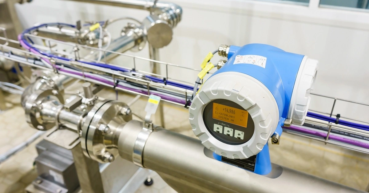
Air compressors are essential in many industries, powering tools, inflating tires, and driving machinery.
Traditional maintenance methods, however, can be slow and costly.
Machine learning enables predictive maintenance, detecting faults early to reduce downtime and extend equipment life.
Contents
1. Application type
We will predict the bearing status in the air compressor system, a binary variable (0 or 1). Therefore, this is a classification project.
The goal here is to model the bearings’ status based on the features of the air compressor system for its subsequent use in predictive maintenance.
2. Data set
For this study, we use a specialized dataset of air compressor systems to train a neural network for predictive maintenance.
The dataset includes key parameters, such as motor RPM, power, torque, outlet pressure, and oil pump power, which capture the system’s operating conditions.
It defines four possible targets—Bearings Status, Water Pump Status, Radiator Status, and Exhaust Valve Status.
In this work, we focus on predicting the Bearings’ Status, though the same method can be applied to the other components.
The first step involves preparing the data set, which serves as the primary source of information for the problem.
There are three main components to configure:
- Data source.
- Variables.
- Instances.
Data source
The data file air_compressor_maintenance.csv contains the information for the air compressor example.
This dataset comprises measurements taken from a compressor system supplying air to a factory production line, with a total of 17 features collected.
The dataset comprises 17 variables (columns) and 1000 instances (rows).
Variables
The features or variables included in the dataset are as follows:
Compressor and motor variables
- RPM – Rotations per minute of the motor.
- Motor Power – Electric motor power consumption (kW).
- Torque – Torque produced by the motor (Nm).
- Outlet Pressure Bar – Compressed air outlet pressure (bar).
- Air Flow – Compressed air flow rate (m³/min).
- Noise dB – Noise level of the compressor (dB).
- Outlet Temp – Outlet temperature of compressed air (°C).
Cooling water system variables
- Water Pump Outlet Pressure – Outlet pressure of the water pump (bar).
- Water Inlet Temp – Inlet temperature of cooling water (°C).
- Water Outlet Temp – Outlet temperature of cooling water (°C).
- Water Pump Power – Water pump power consumption (kW).
- Water Flow – Cooling water flow rate (m³/min).
Oil system variables
- Oil Pump Power – Oil pump power consumption (kW).
- Oil Tank Temp – Oil tank temperature (°C).
Vibration and acceleration variables
- Ground Acceleration – Acceleration at the compressor’s mounting point (X, Y, Z in m/s²).
- Head Acceleration – Acceleration at the compressor head bolt or cooling fin (X, Y, Z in g).
Condition monitoring
- Bearings Status – Condition of the bearings: Ok (normal) or Noise (possible wear/damage).
All variables in the study are inputs, except for the chosen target variable, Bearings Status, which is the output we aim to extract for this machine learning study.
However, if desired, the same methodology could be applied to the other three target variables: Water Pump Status, Radiator Status, and Exhaust Valve Status.
Instances
The instances are divided into training, selection, and testing subsets.
They represent a certain percentage of the original instances and are randomly split.
The exact percentages depend on the chosen data split approach.
Variables distributions
We can perform a few related analytics once the data set has been set.
First, we check the provided information and ensure the data is of high quality.
The data distributions show the bearing condition percentages.

Please note that the actual distributions may vary depending on the nature of the data collected in the air compressor dataset.
Input-target correlations
The input-target correlations may indicate which factors strongly influence the status of the motor and compressor system bearings.

From the chart, we can identify which features have a significant influence on bearing conditions.
This information can help us better understand the relationships between the variables and the target in the predictive maintenance study.
3. Neural network
The second step is to select a neural network that represents the classification function.
For classification problems, it is composed of:
- A scaling layer.
- A dense layer.
Scaling layer
The scaling layer contains the statistics on the input calculated from the data file and the method for scaling the input variables.
The minimum and maximum scaling methods are set here; however, the mean and standard deviation scaling methods yield similar results.
Dense layer
We set just one dense layer with 20 inputs and 1 output, having the logistic activation function.
Neural network graph
The following figure shows the neural network used in this example.
The yellow circles represent scaling neurons, the blue circles represent perceptron neurons, and the red circles represent probabilistic neurons.
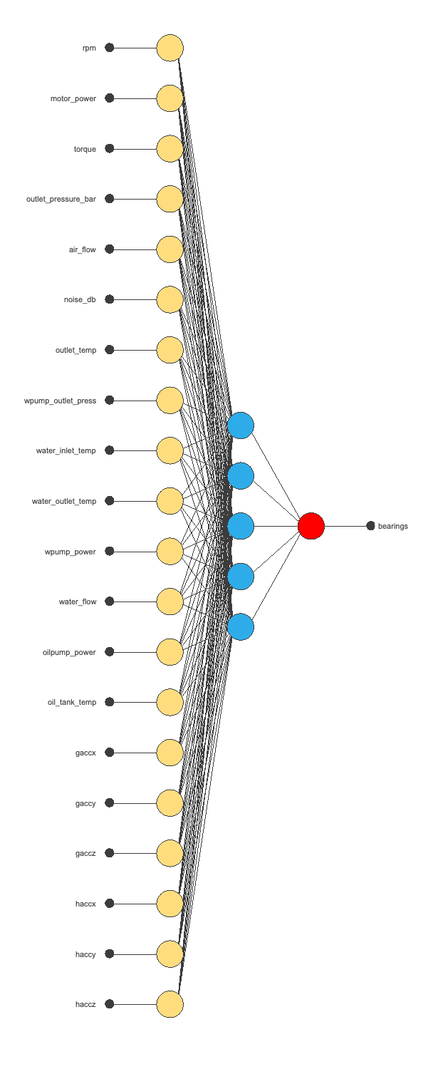
The number of inputs is 20, and the number of outputs is 1.
4. Training strategy
The training strategy is applied to the neural network to obtain the best possible performance. It is composed of two things:
- A loss index.
- An optimization algorithm.
Loss index
The selected loss index is the normalized squared error (NSE) with L2 regularization.
The normalized squared error is helpful in applications where the targets are balanced, as in this case.
The error term fits the neural network to the training instances of the dataset.
The regularization term makes the model more stable and improves generalization, so our model will be more predictive.
Optimization algorithm
The selected optimization algorithm, which minimizes the loss index, is the quasi-Newton method.
Training
The following chart shows how the training (blue) and selection (orange) errors decrease with the training epochs.

The final training and selection errors are a training error of 0.001 NSE (blue) and a selection error of 0.002 NSE (orange), respectively.
Considering the low values of the training and selection errors, the model already demonstrates good performance.
5. Testing analysis
The next step is to perform a test analysis to validate the predictive capability of the neural network.
The next step is to perform a testing analysis to validate the predictive capability of the neural network.
The testing compares the values provided by this technique to the observed values.
ROC curve
The ROC curve is a good measure of the precision of a binary classification model.
Our focus is on evaluating the area under the curve (AUC).
A perfect classifier would have an AUC=1, which implies excellent prediction capabilities, and a random one would have AUC=0.5, indicating no better than random chance.

In this case, our model achieves an AUC of 0.998, indicating that it has practically perfect classification and prediction capabilities.
Confusion matrix
We can also look at the confusion matrix.
Below, we show the elements of this matrix for a decision threshold = 0.43.

Binary classification metrics
From the above confusion matrix, we can calculate the following binary classification tests:
- Accuracy: 99% (ratio of correctly classified samples).
- Error: 1% (ratio of misclassified samples).
- Sensitivity: 98.8% (percentage of actual positives classified as positive).
- Specificity: 100% (percentage of actual negatives classified as negative).
6. Model deployment
Once we have tested the air compressor bearings status classification model, we can use it to evaluate the probability of a specific bearing status.
Neural network outputs
For instance, consider an air compressor with the following features:
- rpm: 1499.52
- motor_power: 6984.88
- torque: 49.186
- outlet_pressure_bar: 4.06
- air_flow: 754.67
- noise_db: 53.41
- outlet_temp: 118.86
- wpump_outlet_press: 2.80
- water_inlet_temp: 83.02
- water_outlet_temp: 96.64
- wpump_power: 222.19
- water_flow: 53.71
- oilpump_power: 300.48
- oil_tank_temp: 46.24
- gaccx: 0.60
- gaccy: 0.35
- gaccz: 3.92
- haccx: 1.10
- haccy: 1.35
- haccz: 3.50
- bearings (1 = OK): 1.00
The probability of ‘OK’ for these bearings is 100%.
References
- Predictive Maintenance Dataset for Air Compressor System by Ahmet Okudan on Kaggle.