This example builds a machine learning model to evaluate the radiation efficiency of patch antennas with different features.
We used data from 8 antennas, including variables extracted from their geometries.
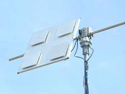
A patch antenna is a type of wireless antenna that utilizes a flat, rectangular metal patch on a substrate to transmit or receive radio frequency (RF) signals.
The coefficient of reflection, S11, measures the power reflected to the source when RF signals are transmitted through the patch antenna.
S11 is typically expressed as a ratio of power, with values close to 0 indicating a small reflection and values close to 1 indicating a significant reflection.
Contents
This dataset was generated using HFSS software, with the radiation frequency set at 2.4 GHz, a frequency commonly used for Bluetooth and WLAN operations, which can be utilized to optimize the design and performance of patch antennas.
1. Application type
The predicted variable in this application is the coefficient of reflection, S11, for a patch antenna.
Therefore, this is an approximation project.
Optimizing the antenna design aims to achieve the lowest possible value for S11, signifying high power transmission and minimal reflection levels, employing artificial intelligence and machine learning.
2. Data set
This dataset features information on patch antennas, a type of microstrip antenna widely used in wireless communications.
The dataset includes various dimensions and parameters of the antenna, including the operating frequency, dimensions of the patch and slots, and a measure of the antenna’s reflection coefficient. The data is organized into 8 clusters.
Variables
The number of input variables, or attributes for each sample, is 7. The target variable is S11.
The following list summarizes the variables’ information:
Antenna Dimensions
- Length of patch (mm): Length of the patch antenna.
- Width of patch (mm): Width of the patch antenna.
- Area of patch (mm²): Total area of the patch antenna.
Slot Dimensions
- Slot length (mm): Length of the antenna slots.
- Slot width (mm): Width of the antenna slots.
- Slot area (mm²): Total area of the antenna slots.
Operating Parameters
- Frequency (GHz): Operating frequency of the antenna.
- Reflection coefficient S11 (dB): The S11 parameter, representing the antenna’s reflection coefficient in decibels.
Instances
Each instance contains the input and target variables of a different patient.
The data set is divided into training, validation, and testing subsets.
Neural Designer automatically assigns 60% of the instances for training, 20% for selection, and 20% for testing.
Correlations
The input-target correlations might indicate which factors have the most significant influence on the reflection coefficient.
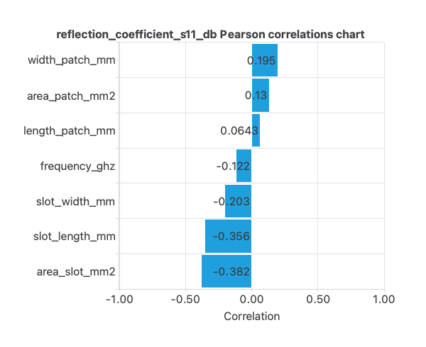
Here, the most correlated variables with survival status are area_slot_mm2 and slot_length_mm.
3. Neural network
The next step is to set up a neural network that represents the approximation function.
For this class of applications, the neural network consists of the following components:
Scaling layer
The scaling layer contains the statistics on the inputs calculated from the data file and the method for scaling the input variables.
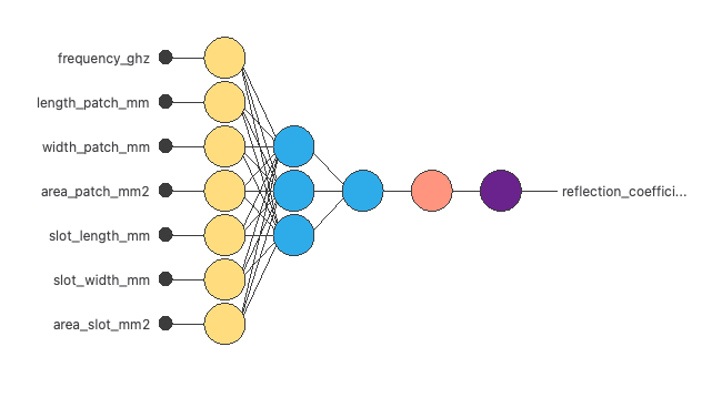
Here, the minimum-maximum method has been set. As we use 7 input variables, the scaling layer has 7 inputs.
Dense layers
We use 2 dense layers here.
The first dense layer has 7 inputs, 3 neurons, and a hyperbolic tangent activation function
The second dense layer has 3 inputs, 1 neuron, and a linear activation function
Unscaling layer
The unscaling layer contains the statistics of the output.
The following figure is a graphical representation of this neural network.
4. Training strategy
The fourth step is to set the training strategy, which is composed of two terms:
- A loss index.
- An optimization algorithm.
Loss index
The loss index is the weighted squared error with L2 regularization, the default loss index for binary classification applications.
We can state the learning problem as finding a neural network that minimizes the loss index.
That is a neural network that fits the data set (error term) and does not oscillate (regularization term).
Optimization algorithm
The optimization algorithm we use is the quasi-Newton method, which is also the standard approach for this type of problem.
The following chart shows how errors decrease with the iterations during training.
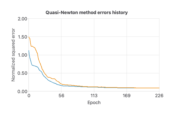
As the previous figure shows, the curves have converged.
5. Testing analysis
The testing analysis aims to validate the generalization properties of the trained neural network.
In this case, we show the minimums, maximums, mean, and standard deviations of the absolute and percent errors of the neural network for the testing data.

As we can see, the average error is around 1%.
Additionally, the error histogram displays the distribution of errors from the neural network on the test samples.
In general, we expect a normal distribution like this.

As we can observe, most of the errors are around 0.
6. Model deployment
Once we have tested the neural network’s generalization performance, we can save it for future use in the so-called model deployment mode.
References
- The data for this problem are available in the Kaggle repository.