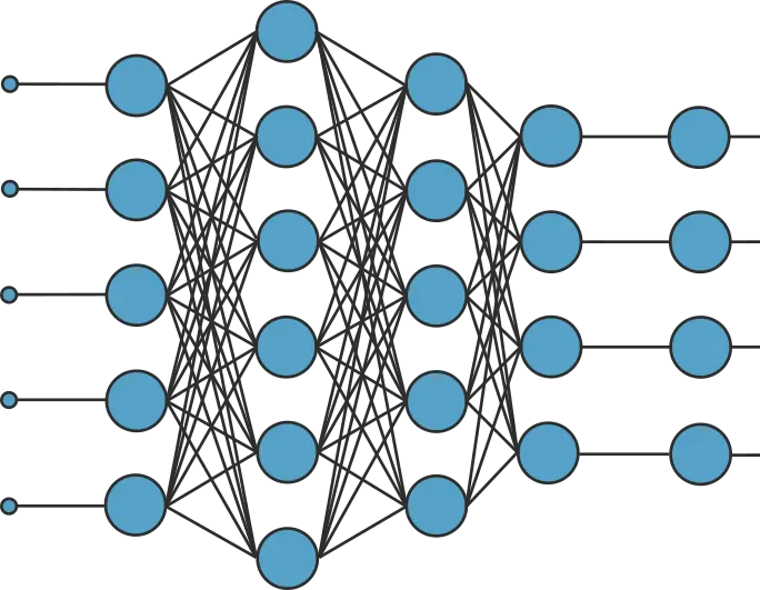
Neural networks are usually arranged as sequences of layers. In turn, layers are made up of individual neurons. Therefore, neurons are the basic information processing units in neural networks.
The most widely used neuron model is the perceptron. This is the neuron model behind perceptron layers (also called dense layers), which are present in the majority of neural networks.
In this post, we explain the mathematics of the perceptron neuron model:
1. Perceptron elements
The following figure is a graphical representation of a perceptron.
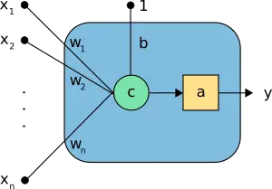
In the above neuron, we can see the following elements:
- The inputs \( \mathbf{x}=(x_1, \ldots, x_n) \).
- The bias \( b \) and the synaptic weights \( \mathbf{w}=(w_1, \ldots, w_n) \).
- The combination function, \( c(\cdot) \) .
- The activation function \( a(\cdot) \) .
- The output y.
For example, consider the neuron in the following figure, with three inputs.
It transforms the inputs \( \mathbf{x}=(x_1,x_2,x_3) \) into a single output \( y \).
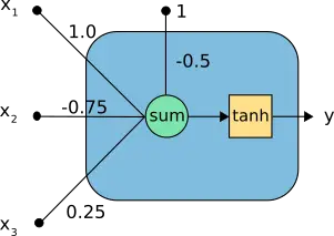
In the above neuron, we can see the following elements:
- The inputs \( \mathbf{x}=(x_1,x_2,x_3) \).
- The neuron parameters, which are the set \( b=-0.5 \) and \( \mathbf{w}=(1.0,-0.75,0.25) \).
- The combination function, \( c(·) \), merges the inputs with the bias and the synaptic weights.
- The activation function, which is set to be the hyperbolic tangent, \( \tanh(\cdot) \) , and takes that combination to produce the output from the neuron.
- The output \( y \).
2. Neuron parameters
The neuron parameters consist of bias and a set of synaptic weights.
- The bias \( b \) is a real number.
- The synaptic weights \( \mathbf{w}=(w_1,\ldots,w_n) \) is a vector of size the number of inputs.
Therefore, the total number of parameters is ( 1+n ), being ( n ) the number of neurons’ inputs.
Consider the perceptron of the example above. That neuron model has a bias and three synaptic weights:
- The bias is \( b = -0.5 \).
- The synaptic weight vector is \( \mathbf{w}=(1.0,-0.75,0.25) \).
The number of parameters in this neuron is ( 1+3=4 ).
3. Combination function
The combination function takes the input vector ( x ) to produce a combined value, or net input, ( c ). The combination is computed as bias plus a linear combination of the synaptic weights and the inputs in the perceptron,
$$
c = \sum_{i=1}^{n} w_i \cdot x_i,
$$
for ( i=1,ldots,n ).
Note that the bias increases or reduces the net input to the activation function, depending on whether it is positive or negative.
The bias is sometimes represented as a synaptic weight connected to an input fixed to ( +1 ).
Consider the neuron of our example.
The combination value of this perceptron for an input vector \( \mathbf{x} = (-0.8,0.2,-0.4) \) is
$$
c = -0.5 + (1.0·-0.8)
+ (-0.75·0.2) + (0.25·-0.4)
= -1.55.
$$
4. Activation function
The activation function defines the output from the neuron in terms of its combination. In practice, we can consider many useful activation functions. Four of the most used are the following:
- Hyperbolic tangent activation.
- Rectified linear (ReLU) activation.
- Linear activation.
- Logistic activation.
Hyperbolic tangent activation
The hyperbolic tangent is defined by
$$
a = tanh{(c)}.
$$
This activation function is represented in the next figure.
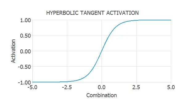
As we can see, the hyperbolic tangent has a sigmoid shape and varies in the range (-1,1). This activation is a monotonous crescent function that perfectly balances linear and non-linear behaviour.
In our example, the combination value is ( c = -1.55 ). As the chosen function is the hyperbolic tangent, the activation of this neuron is
$$
a = tanh{(-1.55)}
= -0.91
$$
The hyperbolic tangent function is very used in the hidden layers of neural networks for approximation and classification tasks.
Rectified linear (ReLU) activation
The rectified linear activation function (also known as ReLU) is another non-linear activation function that has gained popularity in machine learning. The activation is zero for negative combinations. The activation is equal to the combination when the combination is zero or positive.
$$activation = \left\{ \begin{array}{lll}
0 &if& \textrm{$combination < 0$} \\
combination &if& \textrm{$combination \geq 0$}
\end{array} \right. $$
The ReLU function is represented in the next figure.
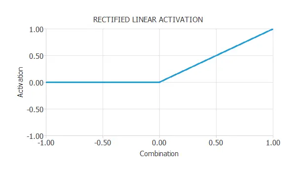
An advantage of the ReLU function is that it is more computationally efficient than other non-linear activation functions,
due to its simplicity. The ReLU function is very used in the hidden layers of neural networks for approximation and classification tasks.
Linear activation
For the linear activation function, we have
$$
a = c
$$
Thus, the output of a neuron with a linear activation function is equal to its combination. The following figure plots the linear activation function.
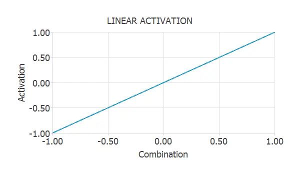
The linear activation function is very used in the output layer of approximation neural networks.
Logistic activation
As the hyperbolic tangent, the logistic function has a sigmoid shape. The logistic function is defined by
$$
a = \frac{1}{1+\exp{(-c)}}.
$$
This activation is represented in the next figure.
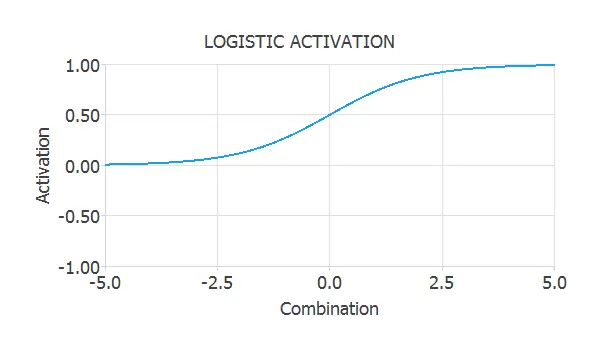
As we can see, the image of the logistic function is ( (0,1) ). This is a suitable property because we can interpret the outputs as probabilities. Therefore, the logistic function is widely used in the output layer of neural networks for binary classification.
5. Output function
The output calculation is the most critical function in the perceptron. Given a set of input signals to the neuron, it computes the output signal from it. The output function is represented in terms of the composition of the combination and the activation functions.
The following figure is an activity diagram of how the information is propagated in the perceptron.
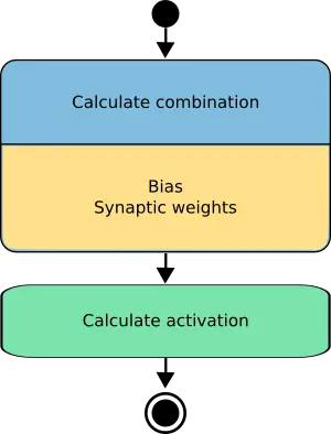
Therefore, the final expression of the output from a neuron as a function of the input to it is
$$
y = a (b+w\cdot x)
$$
Consider the perceptron of our example.
If we apply an input \( \mathbf{x} = (-0.8,0.2,-0.4) \), the output y is the following
$$y = tanh{(-0.5 + (1.0·-0.8) + (-0.75·0.2) + (0.25·-0.4))}
= tanh{(-1.55)}
= -0.91$$
As we can see, the output function merges the combination and the activation functions.
6. Conclusions
A neuron is a mathematical model of the behaviour of a single neuron in a biological nervous system.
A single neuron can solve some simple tasks, but the power of neural networks comes when many of them are arranged in layers and connected in a network architecture.
Although we have seen the functioning of the perceptron in this post, other neuron models have different characteristics and are used for different purposes.
Some of them are the scaling neuron, the principal components neuron, or the unscaling neuron.
Some neuron models only make sense when they are contextualized in a layer and cannot be defined individually. Some of these are the recurrent, long-short term memory (LSTM) or probabilistic layers.