In this example, we build a machine learning model to predict whether the space flights in outer space will be a success or a failure concerning different variables regarding the mission’s nature.

Space missions have changed significantly since the first spacecraft was launched in 1957. They have become incredibly diverse in the current age, with various government agencies, private companies, and international organizations launching missions to explore our solar system and beyond. 

Today, space missions are pushing the boundaries of our knowledge and capabilities in space exploration and technology, focusing on advancing scientific research and understanding and expanding our human presence beyond Earth. 

Contents

1. Application type.
2. Data set.
3. Neural network.
4. Training strategy.
5. Model selection.
6. Testing analysis.
7. Model deployment.

This example is solved with Neural Designer. To follow it step by step, you can use the free trial.

1. Application type

The variable to be predicted is binary. Therefore, this is a classification project.

The main goal is to model the state of the mission as a function of variables such as temperature, nature of the payload, payload target orbit, etc.

2. Data set

The first step is to prepare the data set, which is the source of information for the classification problem. It is composed of:

• Data source.
• Variables.
• Samples.

Data source

The file space_missions.csv contains the data for this example. Here, the number of variables (columns) is 33, and the number of samples (rows) is 166.

Variables

Of the 33 variables, 32 are used as inputs, and the mission status variable is the target variable.

Below, we describe each variable:

• company. Space Company that carried out the space flight. This variable is categorical and there are seven companies: Space X, Boeing, US Air Force, European Space Agency, Brazilian Space Agency, Arianespace, and Martin Marietta.
• temperature_f. Temperature during exact date and deployment time (displayed in Fahrenheit degrees). This variable is numerical, so it doesn’t need any modification.
• wind_speed_mph. Wind speed during exact date and deployment time (displayed in Miles per Hour). This variable is numerical, so it doesn’t need any modification.
• humidity_pct. Humidity during exact date and time of deployment (displayed in percentage). This variable is numerical, so it doesn’t need any modification.
• vehicle_type. In the data set there are six vehicle types. This is also a categorical variable. The vehicle types are Ariane, Delta, Falcon, Titan, VLS and Vega.
• liftoff_thrust_kn. Rocket Liftoff Thrust (displayed in kiloNewtons). This variable is numerical, so it doesn’t need any modification.
• payload_to_orbit_kg. This variable is numerical, so it doesn’t need any modification.
• rocket_height_m. This variable is numerical, so it doesn’t need any modification.
• fairing_diameter_m. Rocket Fairing Diameter (displayed in meters). This variable is numerical, so it doesn’t need any modification.
• payload_mass_kg. This variable is numerical, so it doesn’t need any modification.
• payload_orbit. Orbit to which the payload is programmed to reach. This is a categorical variable as well, the different orbits are Earth-Moon L2, Geostationary Transfer Orbit, Heliocentric Orbit, High Earth Orbit, Medium Earth Orbit, Low Earth Orbit, Mars Orbit, Polar Orbit, Suborbital, Sun-Synchronous Orbit, and Sun/Earth Orbit.
• mission_status. This is the target variable we want to predict. The mission status is either a success or a failure.

Samples

On the other hand, the space_missions.csv data set contains 166 samples. They are divided randomly into training, selection, and testing subsets, including 60%, 20%, and 20% of the instances. More specifically, 90 samples are used here for training, 30 for validation, and 30 for testing.

Once all the data set information has been set, we will perform some analytics to check the quality of the data.

For instance, we can calculate the data distribution. The following figure depicts the pie chart for the target variable.

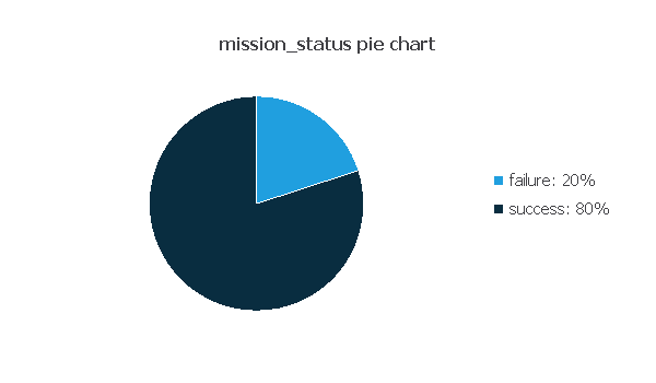
As we can see, the following chart illustrates the target ‘mission_status’ dependency with the 10 input columns with greatest correlation in the data set.

The inputs-targets correlations might help us see the different inputs’ influence on the mission status.

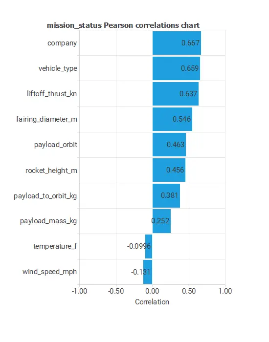
The above chart shows that the company has the most significant impact on the mission status with a correlation to the target variable of 0.667.

3. Neural network

The neural network will output the mission status as a function of the input variables described in the previous section.

For this classification example, the neural network is composed of:

• A scaling layer.
• A perceptron layer.
• A probabilistic layer.

The scaling layer contains the statistics on the input calculated from the data file and the method for scaling the input variables. The minimum and maximum scaling methods are set here, but the mean and standard deviation scaling methods produce similar results.

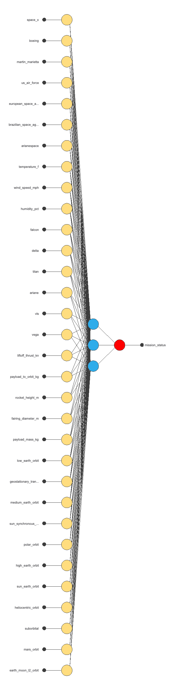
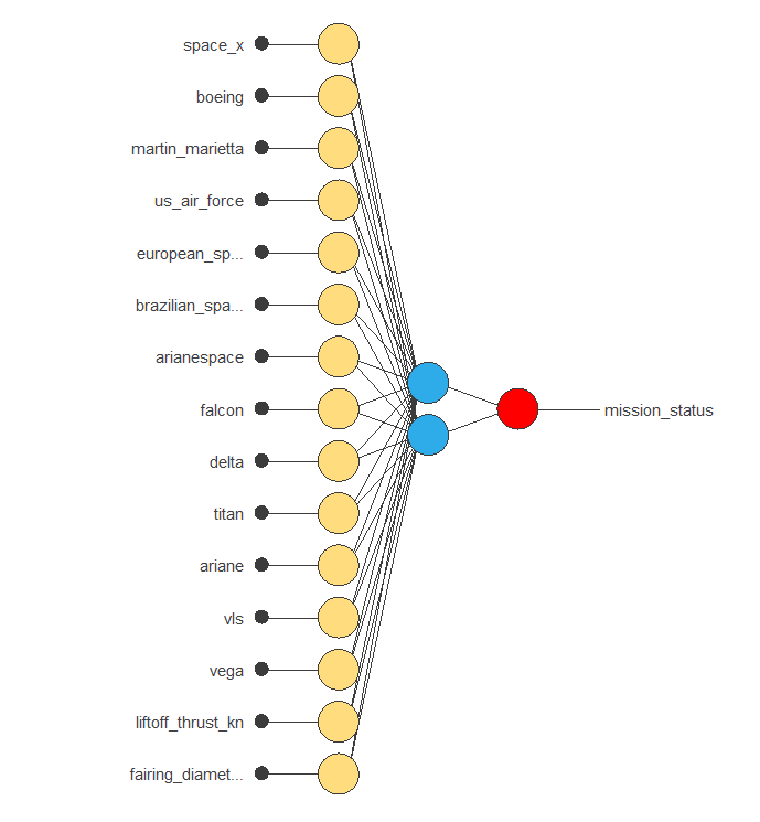
Initially, the number of inputs is 32, and there are 2 neurons in the perceptron layer, with the hyperbolic tangent as the activation function. The generalization study will eliminate variables that do not improve the predictive capabilities of the neural network from the scaling layer. It may also reduce or increase the neurons in the perceptron layer until it finds the optimal complexity.

The next figure is the initial neural network architecture used in this example.

The yellow circles represent scaling neurons, the blue circles perceptron neurons, and the red circles probabilistic neurons. The number of inputs is 32, and the number of outputs is 1.

4. Training strategy

The training strategy is applied to the neural network to obtain the best possible performance. It is composed of two things:

• A loss index.
• An optimization algorithm.

Loss index

The selected loss index is the weighted squared error (WSE) with L2 regularization because, in this problem, the target samples aren’t balanced, as there are more cases where the mission status is 1 than where it’s 0.

The error term fits the neural network to the training instances of the data set. The regularization term makes the model more stable and improves generalization so our model will be more predictive.

Optimization algorithm

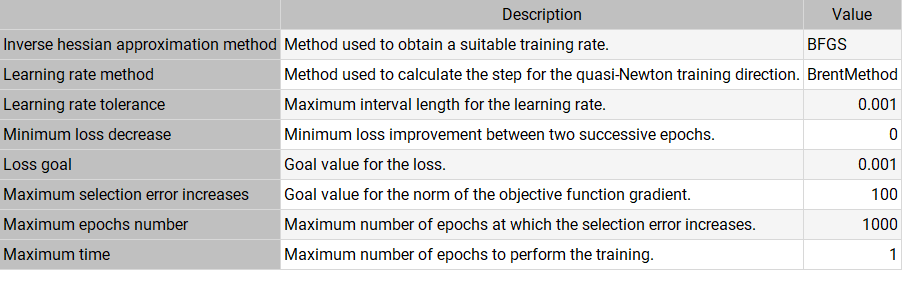
The selected optimization algorithm that minimizes the loss index is the quasi-Newton method.

The following table shows the operators, parameters, and stopping criteria of the quasi-Newton method used in this study.

5. Model selection

The objective of model selection is to find the network architecture with the best generalization properties. That is, we want to improve the final selection error by changing the inputs number or the number of neurons in the perceptron layer.

The best selection error is achieved using a model whose complexity is the most appropriate to produce a better data fit. Order selection algorithms are responsible for finding the optimal number of perceptron neurons in the neural networks.

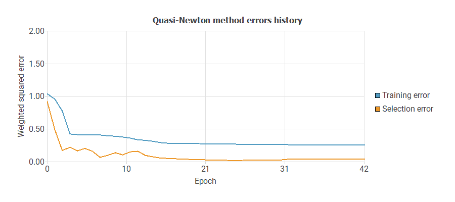
After performing neurons selection and inputs selection, the model is set at optimal 2 neurons in the perceptron layer and 4 inputs in the scaling layer (company, vehicle type, lift-off thrust, and fairing diameter). The following chart shows how the training error (blue) and selection error (orange) decrease with the training epochs.

The final training and selection errors after 42 epochs are training error = 0.259 NSE and selection error = 0.0406 NSE, respectively.

The following figure shows the final network architecture for this application after optimizing our model.

6. Testing analysis

The objective of the testing analysis is to validate the generalization performance of the trained neural network. The testing compares the values provided by this technique to the observed values.

A good measure of the precision of a binary classification model is the ROC curve.

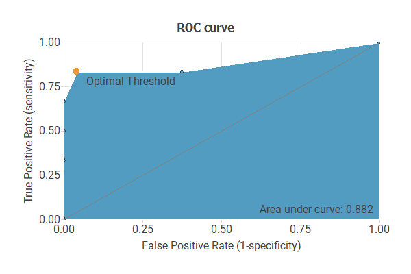
We are interested in the area under the curve (AUC). A perfect classifier would have an AUC=1, and a random one would have an AUC=0.5. Our model has an AUC = 0.882, which is a good indicator of our model.

We can also look at the confusion matrix. Next, we show the elements of this matrix:

From the above confusion matrix, we can calculate the following binary classification tests:

• Classification accuracy: 93.3% (ratio of correctly classified samples).
• Error rate: 6.7% (ratio of misclassified samples).
• Sensitivity:100% (percentage of actual positive classified as positive).
• Specificity: 66.7% (percentage of actual negative classified as negative).

7. Model deployment

After testing, the model is ready to estimate the mission status of new space missions with satisfactory quality over the same data range.

To classify any given star, we calculate the neural network outputs from the different variables: temperature, luminosity, relative radius, absolute magnitude, color, and spectral class. For example, if we introduce the following values for each input:

• Company: boeing
• Vehicle Type: delta
• Liftoff Thrust (kN): 5668.36
• Fairing Diameter (m): 4.25
• Mission status: 0.9=success

The model predicts a mission_status value of 0.9, which means that the mission is a success for those variables.

We can export the mathematical expression listed below.

scaled_space_x = space_x*(1+1)/(1-(0))-0*(1+1)/(1-0)-1;
scaled_boeing = boeing*(1+1)/(1-(0))-0*(1+1)/(1-0)-1;
scaled_martin_marietta = martin_marietta*(1+1)/(1-(0))-0*(1+1)/(1-0)-1;
scaled_us_air_force = us_air_force*(1+1)/(1-(0))-0*(1+1)/(1-0)-1;
scaled_european_space_agency = european_space_agency*(1+1)/(1-(0))-0*(1+1)/(1-0)-1;
scaled_brazilian_space_agency = brazilian_space_agency*(1+1)/(1-(0))-0*(1+1)/(1-0)-1;
scaled_arianespace = arianespace*(1+1)/(1-(0))-0*(1+1)/(1-0)-1;
scaled_falcon = falcon*(1+1)/(1-(0))-0*(1+1)/(1-0)-1;
scaled_delta = delta*(1+1)/(1-(0))-0*(1+1)/(1-0)-1;
scaled_titan = titan*(1+1)/(1-(0))-0*(1+1)/(1-0)-1;
scaled_ariane = ariane*(1+1)/(1-(0))-0*(1+1)/(1-0)-1;
scaled_vls = vls*(1+1)/(1-(0))-0*(1+1)/(1-0)-1;
scaled_vega = vega*(1+1)/(1-(0))-0*(1+1)/(1-0)-1;
scaled_li_ftoff_thrust_kn = (li_ftoff_thrust_kn-5668.359863)/3619.5;
scaled_payload_to_orbit_kg = (payload_to_orbit_kg-10708.90039)/9502.620117;
scaled_rocket_height_m = (rocket_height_m-56.33710098)/16.57769966;
scaled_fairing_diameter_m = (fairing_diameter_m-4.252329826)/1.291180015;
scaled_low_earth_orbit = low_earth_orbit*(1+1)/(1-(0))-0*(1+1)/(1-0)-1;
scaled_geostationary_transfer_orbit = geostationary_transfer_orbit*(1+1)/(1-(0))-0*(1+1)/(1-0)-1;
scaled_medium_earth_orbit = medium_earth_orbit*(1+1)/(1-(0))-0*(1+1)/(1-0)-1;
scaled_sun_synchronous_orbit = sun_synchronous_orbit*(1+1)/(1-(0))-0*(1+1)/(1-0)-1;
scaled_polar_orbit = polar_orbit*(1+1)/(1-(0))-0*(1+1)/(1-0)-1;
scaled_high_earth_orbit = high_earth_orbit*(1+1)/(1-(0))-0*(1+1)/(1-0)-1;
scaled_sun_earth_orbit = sun_earth_orbit*(1+1)/(1-(0))-0*(1+1)/(1-0)-1;
scaled_heliocentric_orbit = heliocentric_orbit*(1+1)/(1-(0))-0*(1+1)/(1-0)-1;
scaled_suborbital = suborbital*(1+1)/(1-(0))-0*(1+1)/(1-0)-1;
scaled_mars_orbit = mars_orbit*(1+1)/(1-(0))-0*(1+1)/(1-0)-1;
scaled_earth_moon_l_two__orbit = earth_moon_l_two__orbit*(1+1)/(1-(0))-0*(1+1)/(1-0)-1;

perceptron_layer_1_output_0 = tanh( -0.0252279 + (scaled_space_x*-0.977736) + (scaled_boeing*-1.85103) + (scaled_martin_marietta*0.314955) + (scaled_us_air_force*0.510748) + (scaled_european_space_agency*0.556204) + (scaled_brazilian_space_agency*0.377423) + (scaled_arianespace*1.3211) + (scaled_falcon*-1.17816) + (scaled_delta*-1.91861) + (scaled_titan*0.745279) + (scaled_ariane*1.72617) + (scaled_vls*0.350494) + (scaled_vega*0.294097) + (scaled_li_ftoff_thrust_kn*-0.39278) + (scaled_payload_to_orbit_kg*-0.746857) + (scaled_rocket_height_m*-1.94832) + (scaled_fairing_diameter_m*-0.1606) + (scaled_low_earth_orbit*-0.0151092) + (scaled_geostationary_transfer_orbit*1.39765) + (scaled_medium_earth_orbit*-0.469048) + (scaled_sun_synchronous_orbit*-0.132675) + (scaled_polar_orbit*-0.28124) + (scaled_high_earth_orbit*0.382293) + (scaled_sun_earth_orbit*0.0238606) + (scaled_heliocentric_orbit*-0.390002) + (scaled_suborbital*0.122364) + (scaled_mars_orbit*0.0601759) + (scaled_earth_moon_l_two__orbit*-0.0988727) );
perceptron_layer_1_output_1 = tanh( -0.398011 + (scaled_space_x*0.213628) + (scaled_boeing*0.278193) + (scaled_martin_marietta*0.156167) + (scaled_us_air_force*0.447462) + (scaled_european_space_agency*0.280253) + (scaled_brazilian_space_agency*0.200911) + (scaled_arianespace*0.225519) + (scaled_falcon*0.323436) + (scaled_delta*0.125297) + (scaled_titan*0.248663) + (scaled_ariane*-0.107428) + (scaled_vls*0.229402) + (scaled_vega*0.490182) + (scaled_li_ftoff_thrust_kn*-0.169335) + (scaled_payload_to_orbit_kg*-0.0174265) + (scaled_rocket_height_m*0.0234038) + (scaled_fairing_diameter_m*0.0217114) + (scaled_low_earth_orbit*-0.0850102) + (scaled_geostationary_transfer_orbit*-0.049046) + (scaled_medium_earth_orbit*0.596493) + (scaled_sun_synchronous_orbit*0.334548) + (scaled_polar_orbit*0.313131) + (scaled_high_earth_orbit*0.366025) + (scaled_sun_earth_orbit*0.264975) + (scaled_heliocentric_orbit*0.514286) + (scaled_suborbital*0.200978) + (scaled_mars_orbit*0.483998) + (scaled_earth_moon_l_two__orbit*0.264058) );
perceptron_layer_1_output_2 = tanh( 0.00878603 + (scaled_space_x*1.4239) + (scaled_boeing*1.24983) + (scaled_martin_marietta*-0.220728) + (scaled_us_air_force*-0.565039) + (scaled_european_space_agency*-0.656933) + (scaled_brazilian_space_agency*-0.267812) + (scaled_arianespace*-1.40038) + (scaled_falcon*1.47574) + (scaled_delta*1.38662) + (scaled_titan*-0.992553) + (scaled_ariane*-1.42127) + (scaled_vls*-0.33815) + (scaled_vega*-0.0876438) + (scaled_li_ftoff_thrust_kn*0.871388) + (scaled_payload_to_orbit_kg*-0.406341) + (scaled_rocket_height_m*1.46813) + (scaled_fairing_diameter_m*-1.02511) + (scaled_low_earth_orbit*0.368851) + (scaled_geostationary_transfer_orbit*-2.40824) + (scaled_medium_earth_orbit*0.438215) + (scaled_sun_synchronous_orbit*0.105603) + (scaled_polar_orbit*0.501919) + (scaled_high_earth_orbit*-0.486344) + (scaled_sun_earth_orbit*-0.0574304) + (scaled_heliocentric_orbit*0.500275) + (scaled_suborbital*-0.118632) + (scaled_mars_orbit*-0.0999855) + (scaled_earth_moon_l_two__orbit*0.131234) );
perceptron_layer_1_output_3 = tanh( -0.365152 + (scaled_space_x*-0.564681) + (scaled_boeing*0.768721) + (scaled_martin_marietta*0.428639) + (scaled_us_air_force*0.113359) + (scaled_european_space_agency*0.368281) + (scaled_brazilian_space_agency*0.387325) + (scaled_arianespace*0.455199) + (scaled_falcon*-0.416892) + (scaled_delta*0.768637) + (scaled_titan*0.273135) + (scaled_ariane*0.492591) + (scaled_vls*0.0717685) + (scaled_vega*0.440991) + (scaled_li_ftoff_thrust_kn*-0.783723) + (scaled_payload_to_orbit_kg*1.02784) + (scaled_rocket_height_m*-0.088811) + (scaled_fairing_diameter_m*1.80013) + (scaled_low_earth_orbit*0.332023) + (scaled_geostationary_transfer_orbit*1.78202) + (scaled_medium_earth_orbit*-0.180319) + (scaled_sun_synchronous_orbit*-0.0815789) + (scaled_polar_orbit*-0.288403) + (scaled_high_earth_orbit*0.468681) + (scaled_sun_earth_orbit*0.384037) + (scaled_heliocentric_orbit*-0.00402607) + (scaled_suborbital*0.271606) + (scaled_mars_orbit*0.344459) + (scaled_earth_moon_l_two__orbit*0.314375) );

probabilistic_layer_combinations_0 = -1.2074 -2.16881*perceptron_layer_1_output_0 +4.01392*perceptron_layer_1_output_1 +2.19242*perceptron_layer_1_output_2 -2.63496*perceptron_layer_1_output_3 
	
mission_status = 1.0/(1.0 + exp(-probabilistic_layer_combinations_0) );

We can implement this expression in any programming language to obtain the output for our input.

References

• Space missions data set from Kaggle repository.

Related posts