Introduction
Machine learning can help predict 5-year mortality risk in breast cancer, a heterogeneous disease influenced by clinical features, treatment, and genomic profiles.
Using the METABRIC dataset of 1,880 patients, a neural network achieved an AUC of 0.8 and 81.4% accuracy, demonstrating its potential as a predictive tool.
Clinicians can test this approach by downloading Neural Designer.
Contents
1. Model type
- Problem type: Binary classification (death or survival)
- Goal: Model the probability of a patient dying from breast cancer based on clinical data, gene expression, and mutational profile to support clinical decision-making.
2. Data set
Data source
The dataset includes 1,880 instances and 689 variables, comprising 26 clinical variables, 489 gene expression variables, and 173 mutation variables.
Variables
The following list summarizes the variables used in the breast cancer mortality prediction model:
Patient information
patient_id – Unique patient identifier.
age_at_diagnosis – Patient’s age at the time of diagnosis (years).
inferred_menopausal_state – Inferred menopausal status: premenopausal or postmenopausal.
Treatment
type_of_breast_surgery – Type of breast surgery: mastectomy, lumpectomy, etc.
chemotherapy (0 or 1) – Indicates whether the patient received chemotherapy.
hormone_therapy (0 or 1) – Indicates whether the patient received hormone therapy.
radio_therapy (0 or 1) – Indicates whether the patient received radiotherapy.
Tumor characteristics
- cancer_type_detailed – Detailed cancer type (e.g., CDIM, NEUTRAL).
- cellularity – Tumor cellularity level (e.g., high, low, NA).
- neoplasm_histologic_grade (1-3) – Histologic grade n of the tumor based on cellular differentiation.
- her2_status (0 or 1) – HER2 status: negative (0) or positive (1).
- her2 status measured by snp6 – Method for measuring HER2 status using SNP6.
- er_status (0 or 1) – Estrogen receptor (ER) status: negative (0) or positive (1).
- er_status_measured_by_ihc – Method for measuring ER status using IHC.
- pr_status – Progesterone receptor (PR) status.
- tumor other histologic subtype – Aditional histologic tumor subtype (e.g., Ductal/NST).
- integrative_cluster – Integrative cluster classification of the tumor.
- primary_tumor_laterality – Primary tumor location (right or left).
- lymph nodes examined positive – Number of lymph nodes examined and positive.
- tumor_size – Tumor size (mm or cm, depending on the dataset).
- tumor_stage – Tumor stage according to TNM or clinical classification.
Genomic features
mutation_count – Total number of mutations detected in the tumor.
pam50_+_claudin-1_subtype – Molecular subtype according to PAM50 + Claudin-1.
3-gene_classifier_subtype – Molecular subtype according to 3-gene classifier.
nottingham prognostic index – Nottingham Prognostic Index calculated from tumor size, lymph nodes, and histologic grade.
Cohort information
- cohort – Cohort to which the patient belongs.
Target variable
- mortality – Can be defined according to the prediction objective (e.g., survival, treatment response, recurrence).
Instances
The dataset’s instances are split into training (60%), validation (20%), and testing (20%) subsets by default.
You can adjust them as needed.
Variables distributions
We can examine variable distributions; the figure shows a pie chart of patients who survived versus those who did not, summarizing mortality in the dataset.
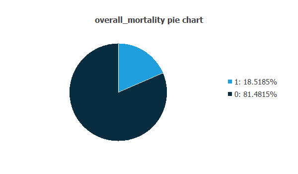
As depicted in the image, 18.52% of the patients did not survive, while approximately 81.48% of the patients survived.
Input-target correlations
The input-target correlations indicate which factors most influence patient mortality and, therefore, are more relevant to our analysis.
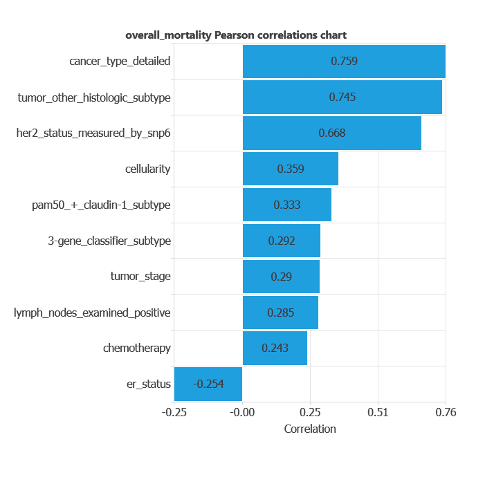
Here, the most correlated variables with mortality are cancer type, detailed tumor other histologic subtype, and HER2 status measured by SNP6.
3. Neural network
A neural network is an artificial intelligence model inspired by how the human brain processes information.
It is organized in layers: the input layer receives the variables, and the output layer provides the probability of belonging to a given class.
Trained with historical data, the network learns to recognize patterns and distinguish between categories, offering objective support for decision-making.
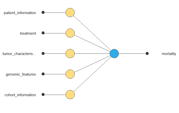
The network uses multiple clinical and demographic variables to output the probability of breast cancer mortality, showing each variable’s contribution to the prediction.
4. Training strategy
Training a neural network involves using a loss function to measure errors and an optimization algorithm to adjust the model, ensuring it learns from data while avoiding overfitting for good performance on new cases.
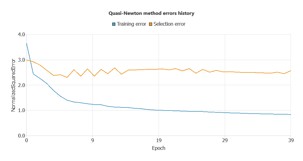
Since the training error is 0.838 and the selection error is higher (2.569), input selection will be applied to reduce overfitting and improve model generalization.
Due to the high number of input neurons and relatively low evaluation metrics, a neuron selection process was performed.
The selection method trains several network architectures with varying numbers of neurons and identifies the configuration that achieves the lowest selection error.
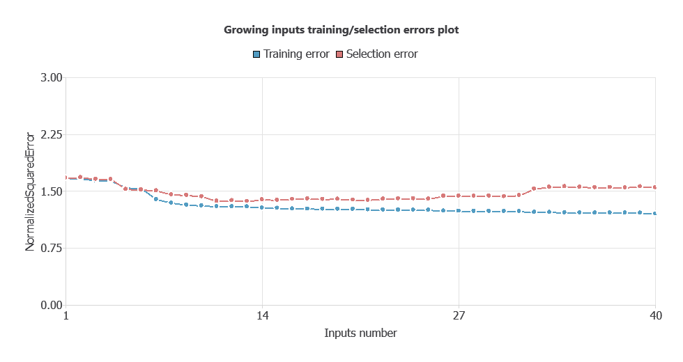
After performing input selection, the model was reduced to 35 inputs (removing less relevant features), which lowered the selection error and simplified the network architecture.
As shown in the chart, both training error and selection error decrease as the number of inputs is optimized, resulting in a more efficient network with improved performance.
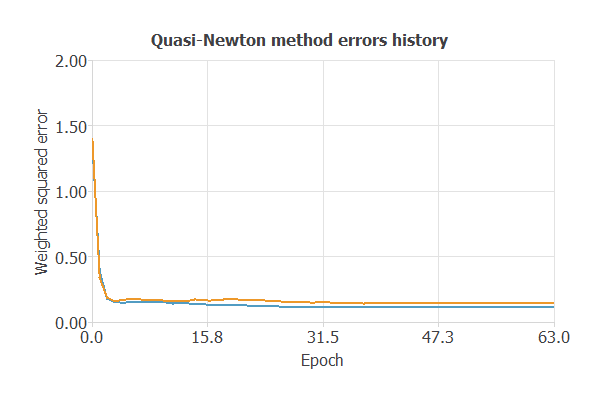
The new model was trained for accuracy and stability, with steadily decreasing training and selection errors (0.115 and 0.143 WSE), demonstrating effective learning and strong generalization to new patients.
6. Testing analysis
The testing analysis aims to validate the performance of the generalization properties of the trained neural network.
ROC curve
The ROC curve is a standard tool to evaluate a classification model, showing how well it distinguishes between two classes by comparing predicted results with actual outcomes, such as survival or mortality.
A random classifier scores 0.5, while a perfect classifier scores 1.
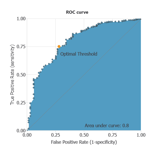
The AUC obtained is 0.8, showing that the model performs exceptionally well at distinguishing between patients who survived and those who did not.
Confusion matrix
The confusion matrix shows the model’s performance by comparing predicted and actual outcomes. It includes:
True positives – patients correctly predicted as deceased
False positives – patients incorrectly predicted as deceased
False negatives – patients incorrectly predicted as surviving
True negatives – patients correctly predicted as surviving
For a decision threshold of 0.5, the confusion matrix was:
| Predicted positive | Predicted negative | |
|---|---|---|
| Real positive | 43 | 29 |
| Real negative | 41 | 263 |
In this case, 81.4% of cases were correctly classified and 18.6% were misclassified.
Binary classification
Using a classification threshold of 0.3, the performance of this binary classification model is summarized with standard measures.
Accuracy: 81.4% of patient outcomes were correctly predicted.
Error rate: 18.6% of cases were misclassified.
Sensitivity: 59.7% of deceased patients were correctly identified.
Specificity: 86.5% of surviving patients were correctly identified.
These measures indicate that the model is highly effective at predicting patient survival outcomes.
7. Model deployment
Once validated, the neural network can be saved for deployment, allowing clinicians to use patients’ clinical data to predict breast cancer mortality.
Neural Designer automatically exports the trained model, enabling seamless integration as a diagnostic support tool.
Conclusions
The breast cancer 5-year mortality prediction model (METABRIC dataset) showed strong performance (AUC = 0.8, accuracy = 81.4%).
Key predictors—lymph nodes examined, tumor stage, ER status, and MAPT gene expression—align with clinical knowledge, supporting reliability.
The model can help clinicians assess mortality risk, complement traditional prognostic tools, and guide treatment decisions.
References
- We have obtained the data for this problem from the cBioportal Repository Cancer (METABRIC, Nature 2012 & Nat Commun 2016) dataset.
- The NEMHESYS – NGS Establishment in Multidisciplinary Healthcare Education System project funded the development of this application.