Introduction
Machine learning for diabetic retinopathy risk prediction aids early detection, enabling timely interventions and reducing vision loss. Accurate prognosis from routine clinical and lab data is challenging.
We developed a neural network model using age, systolic blood pressure, and cholesterol from 6,000 patients, achieving an AUC = 0.75 and 74.3% accuracy. This demonstrates its potential as a clinical decision-support tool.
Healthcare professionals can test this approach with Neural Designer
Contents
The following index outlines the steps for performing the analysis.
1. Model type
In this example, we develop a binary classification model to estimate the probability that a patient will develop diabetic retinopathy. Specifically, the model predicts whether the outcome is 0 (no retinopathy) or 1 (retinopathy).
By framing the problem as a classification task, we allow the neural network to learn patterns associated with higher or lower risk levels. Consequently, clinicians can use the model output as decision-support information.
2. Data set
Data source
The diabetic_retinopathy.csv dataset (6,000 instances, 6 variables) for a binary classification problem (target: 0 = no diabetic retinopathy, 1 = diabetic retinopathy).
Variables
The following list summarizes the variables’ information:
Patient features
age – Age of the patient in years.
systolic_bp – Systolic blood pressure in mmHg.
diastolic_bp – Diastolic blood pressure in mmHg.
cholesterol – Cholesterol level in mg/dL.
Target variable
- retinopathy – Indicates whether the patient develops diabetic retinopathy.
Instances
By default, the dataset is split into 60% training (3,600 samples) and 20% each for validation and testing (1,200 samples combined).
You can adjust proportions if needed.
Variables distributions
Variable distributions can be calculated, and the pie chart shows the number of patients with and without diabetic retinopathy.
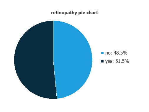
Approximately 48.55% of patients have diabetic retinopathy, while 51.45% do not.
Input-target correlations
The input-target correlations indicate which patient features most influence the development of diabetic retinopathy and, therefore, are most relevant to our analysis.
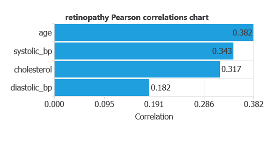
Here, the most correlated variables with malignant tumors are age, systolic bp, and cholesterol.
3. Neural network
A neural network is an artificial intelligence model inspired by how the human brain processes information.
It is organized in layers: the input layer receives the variables, and the output layer provides the probability of belonging to a given class.
Trained with historical data, the network learns to recognize patterns and distinguish between categories, offering objective support for decision-making.
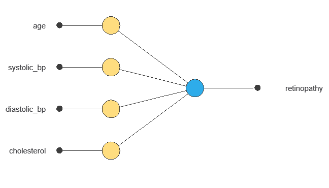
The network uses five patient variables—age, systolic and diastolic blood pressure, cholesterol, and ID—to predict the probability of developing diabetic retinopathy, with connections showing each variable’s contribution.
4. Training strategy
Training a neural network uses a loss function to measure errors and an optimization algorithm to adjust the model, ensuring it learns from data while avoiding overfitting for good performance on new cases.
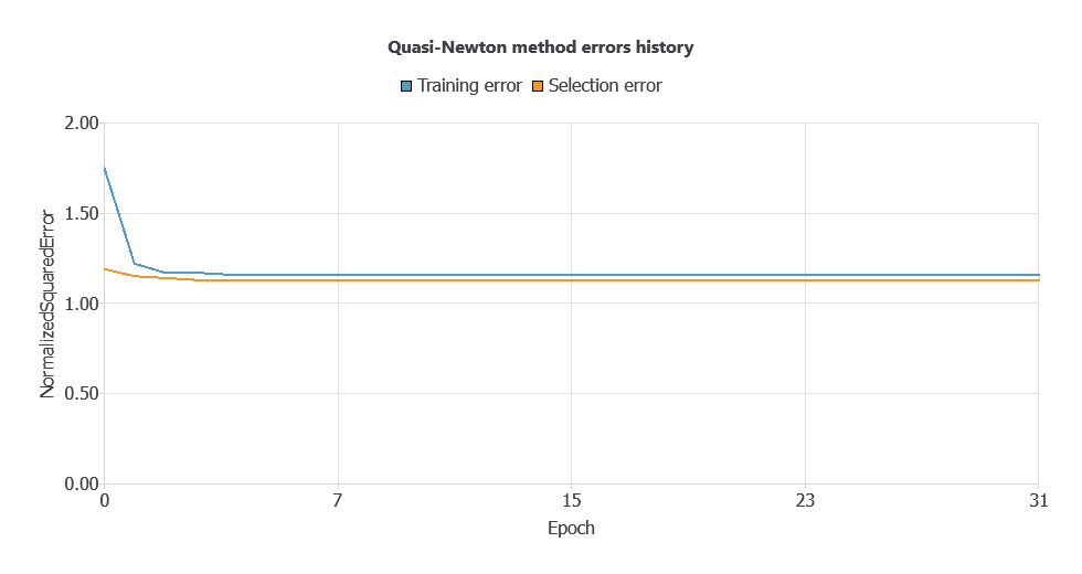
The model was trained for accuracy and stability, with training and validation errors decreasing steadily (1.147 and 1.156 WSE), indicating effective learning and generalization to new patients.
5. Testing analysis
The objective of the testing analysis is to validate the generalization performance of the trained neural network.
ROC curve
The ROC curve is a standard tool to evaluate a classification model, showing how well it distinguishes between two classes by comparing predicted results with actual outcomes, such as patients with or without diabetic retinopathy.
A random classifier scores 0.5, while a perfect classifier scores 1.
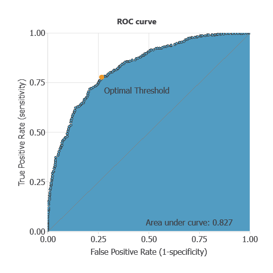
The AUC obtained is 0.826, showing that the model performs well at distinguishing between patients with and without diabetic retinopathy.
Confusion matrix
The confusion matrix shows the model’s performance by comparing predicted and actual outcomes. It includes:
True positives – patients correctly predicted as having diabetic retinopathy
False positives – patients incorrectly predicted as having diabetic retinopathy
False negatives – patients with diabetic retinopathy incorrectly predicted as healthy
True negatives – patients correctly predicted as not having diabetic retinopathy
For a decision threshold of 0.5, the confusion matrix was:
| Predicted positive | Predicted negative | |
|---|---|---|
| Real positive | 464 | 153 |
| Real negative | 150 | 433 |
In this case, 74.75% of cases were correctly classified and 25.25% were misclassified.
Binary classification
The performance of this binary classification model is summarized with standard measures:
Accuracy: 74.8% of patients were correctly classified.
Error rate: 25.3% of cases were misclassified.
Sensitivity: 75.2% of patients with diabetic retinopathy were correctly identified.
Specificity: 74.3% of patients without diabetic retinopathy were correctly identified.
These measures indicate that the model is effective at distinguishing between patients who will develop diabetic retinopathy and those who will not.
6. Model deployment
After confirming the neural network’s ability to generalize, the model can be saved for future use in deployment mode.
This allows the trained network to be applied to new patients, using their clinical and laboratory variables to calculate the probability of developing diabetic retinopathy.
In deployment mode, healthcare professionals can use the model as a reliable diagnostic support tool for classifying new patients.
The Neural Designer software exports the trained model automatically, making it easy to integrate into clinical practice.
Conclusions
The diabetic retinopathy prognosis model, developed with the Coursera dataset, achieved good performance (AUC = 0.75, accuracy = 74.3%) in predicting disease risk.
Key variables—age, systolic blood pressure, and cholesterol—align with clinical knowledge, supporting the model’s reliability.
Its strong generalization makes it a valuable decision-support tool for early risk assessment, complementing clinical evaluations and enabling timely interventions to prevent vision loss.
References
- The data for this problem has been taken from the Coursera repository.