Although deploying a model once trained is essential to benefit from working with Machine Learning, it can also be one of the hardest tasks to accomplish.

Neural Designer includes a series of functionalities that will help you implement this deployment by providing the outputs for a series of inputs of the code or mathematical expression of the model so that you can integrate it in a data pipeline or a Bussiness Intelligence application.

This tutorial will export a Neural Designer model to Python and then integrate it in Power BI.

The data for this application can be obtained from the concrete_properties.csv file. The final Power BI file can be downloaded from concrete_properties.pbix.

To solve this application, the next steps are followed:

  1. Export the model to Python.
  2. Integrate the model in Power BI.

1. Export the model to Python

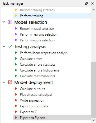
After training our approximation model as seen in the Build a Neural Network in 7 steps tutorial, we will proceed to export that model to Python. You will find the task at the bottom of the Task manager, under the Model deployment section.

This option will allow you to save a .py file with your training model ready for use.
If you open this file in your Python editor, you will find some documentation on using it on top.

Artificial Intelligence Techniques SL
artelnics@artelnics.com
Your model has been exported to this python file.
You can manage it with the 'NeuralNetwork' class.
Example:

	model = NeuralNetwork()
	sample = [input_1, input_2, input_3, input_4, ...]
	outputs = model.calculate_output(sample)

	Inputs Names:
	1 )cement
	2 )blast_furnace_slag
	3 )fly_ash
	4 )water
	5 )superplasticizer
	6 )coarse_aggregate
	7 )fine_aggregate

You can predict with a batch of samples using calculate_batch_output method
IMPORTANT: input batch must be class 'numpy.ndarray' type
Example_1:
	model = NeuralNetwork()
	input_batch = np.array([[1, 2], [4, 5]], np.int32)
	outputs = model.calculate_batch_output(input_batch)
Example_2:
	input_batch = pd.DataFrame( {'col1': [1, 2], 'col2': [3, 4]})
	outputs = model.calculate_batch_output(input_batch.values)
'''

import numpy as np

class NeuralNetwork:

	def __init__(self):

		self.parameters_number = 10

	def scaling_layer(self,inputs):

		outputs = [None] * 7

		outputs[0] = (inputs[0]-265.4440002)/104.6699982
		outputs[1] = (inputs[1]-86.28520203)/87.82649994
		outputs[2] = (inputs[2]-62.79529953)/66.22769928
		outputs[3] = (inputs[3]-183.0599976)/19.32859993
		outputs[4] = (inputs[4]-6.995759964)/5.392280102
		outputs[5] = (inputs[5]-956.059021)/83.8015976
		outputs[6] = (inputs[6]-764.3770142)/73.12049866

		return outputs;


	def perceptron_layer_1(self,inputs):

		combinations = [None] * 1

		combinations[0] = -0.0483297 -0.611001*inputs[0] -0.456874*inputs[1] -0.261702*inputs[2] +0.0291907*inputs[3] -0.0406589*inputs[4] -0.132526*inputs[5] -0.149657*inputs[6]

		activations = [None] * 1
		activations[0] = np.tanh(combinations[0])
		return activations;


	def perceptron_layer_2(self,inputs):

		combinations = [None] * 1
		combinations[0] = -0.0484288 -2.26703*inputs[0]
		activations = [None] * 1
		activations[0] = combinations[0]
		return activations;


	def unscaling_layer(self,inputs):

		outputs = [None] * 1
		outputs[0] = inputs[0]*14.71109962+36.74860001
		return outputs


	def bounding_layer(self,inputs):

		outputs = [None] * 1
		outputs[0] = inputs[0]
		return outputs


	def calculate_output(self, inputs):

		output_scaling_layer = self.scaling_layer(inputs)
		output_perceptron_layer_1 = self.perceptron_layer_1(output_scaling_layer)
		output_perceptron_layer_2 = self.perceptron_layer_2(output_perceptron_layer_1)
		output_unscaling_layer = self.unscaling_layer(output_perceptron_layer_2)
		output_bounding_layer = self.bounding_layer(output_unscaling_layer)
		return output_bounding_layer


	def calculate_batch_output(self, input_batch):

		output = []

		for i in range(input_batch.shape[0]):

			inputs = list(input_batch[i])
			output_scaling_layer = self.scaling_layer(inputs)
			output_perceptron_layer_1 = self.perceptron_layer_1(output_scaling_layer)
			output_perceptron_layer_2 = self.perceptron_layer_2(output_perceptron_layer_1)
			output_unscaling_layer = self.unscaling_layer(output_perceptron_layer_2)
			output_bounding_layer = self.bounding_layer(output_unscaling_layer)
			output = np.append(output,output_bounding_layer, axis=0)

		return output
     

Once we have this code, we can open Power BI to make the deployment.

2. Integrate the model in Power BI

In this case, we will be implementing a Power BI report that shows the output calculated by the model for a series of input values and the directional outputs given for those same values.

We will be working with variables’ parameters, so there is no need to load any dataset. To get the values of those parameters from the user, we will create a slider for each of the input variables.
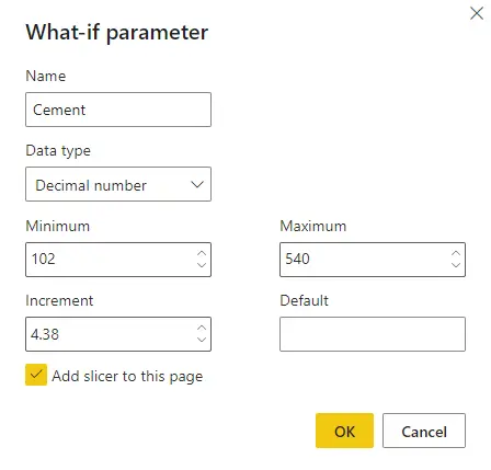
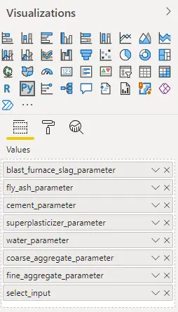
We will click on New Parameter on the modeling tab to create these sliders. There we will use the range of the variable and, as step, the value that gives us 100 steps for such range.

Once we create the sliders for all the inputs, we stack them for easier access.

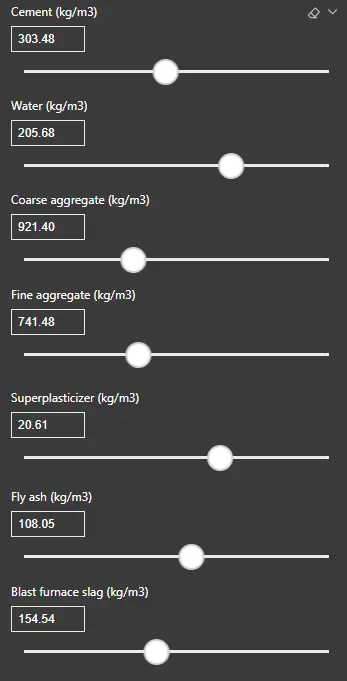
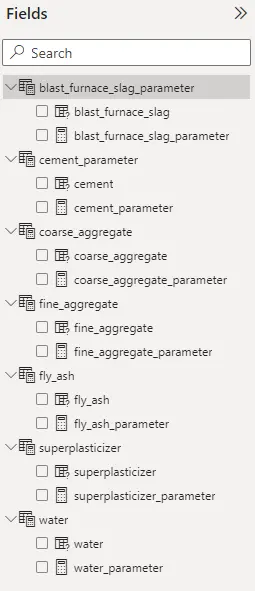
We will name the parameter fields as follows to later work with them in Python.

To calculate the target value, we will be using the Python visual functionality, which allows us to embed a Python script in Power BI. We use the code exported by Neural Designer to calculate the output and, then we plot it so that it can be seen on our report.
The code added to the model is:

import numpy as np
import pandas as pd
import matplotlib.pyplot as plt
import matplotlib.patheffects as path_effects

model = NeuralNetwork()

# Parameter point
input_parameters = [dataset.cement_parameter, dataset.blast_furnace_slag_parameter, dataset.fly_ash_parameter, dataset.water_parameter, dataset.superplasticizer_parameter, dataset.coarse_aggregate_parameter, dataset.fine_aggregate_parameter]

output_point = round(model.calculate_output(input_parameters)[0][0],2)


fig = plt.figure(figsize=(60, 10))
fig.patch.set_facecolor('#3A3A3A')
text = fig.text(0, 0.5, str(output_point) + ' MPa',
                ha='left', va='center', size=500, color ='#d04f25')            
text.set_path_effects([path_effects.Normal()])
plt.show()
     

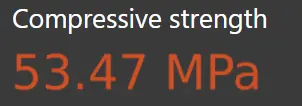
This way, after adding a text box with the name of the target variable, we get the Neural Network’s output.

Next, we will create the directional outputs for each of the inputs. To save some space, we will use a dropdown menu to select the input the user wants to visualize.

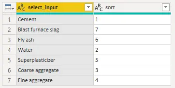
First of all, we have to create a new data table with the names of the variables and the order we want them to appear in.

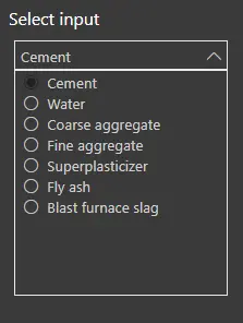
Then, we create a dropdown slicer by clicking on the slicer icon in the visualization section and selecting the inputs column in the table we just created.

Now, we will add another python visual to create the directional output plots. We will use all the inputs’ parameters and the dropdown slicer as values for this visual.

Just as we did while calculating the output, we paste the exported model and add some code to show the plots.
The code added to the model is the one that follows:

import numpy as np
import pandas as pd
import matplotlib.pyplot as plt

model = NeuralNetwork()

points = 100

cement_min = 102
cement_max = 540
blast_furnace_slag_min = 0
blast_furnace_slag_max = 359.4
fly_ash_min = 0
fly_ash_max = 200.1
water_min = 121.8
water_max= 247
superplasticizer_min = 0
superplasticizer_max = 32.2
coarse_aggregate_min = 801
coarse_aggregate_max = 1145
fine_aggregate_min = 594
fine_aggregate_max = 992.6

cement = np.full((1,points),dataset.cement_parameter, dtype = float)[0]
blast_furnace_slag = np.full((1,points),dataset.blast_furnace_slag_parameter, dtype = float)[0]
fly_ash = np.full((1,points),dataset.fly_ash_parameter, dtype = float)[0]
water = np.full((1,points),dataset.water_parameter, dtype = float)[0]
superplasticizer = np.full((1,points),dataset.superplasticizer_parameter, dtype = float)[0]
coarse_aggregate = np.full((1,points),dataset.coarse_aggregate_parameter, dtype = float)[0]
fine_aggregate = np.full((1,points),dataset.fine_aggregate_parameter, dtype = float)[0]

if dataset.select_input[0] == 'Cement':
    cement = np.arange(cement_min ,cement_max, (cement_max-cement_min)/points)
elif dataset.select_input[0] == 'Blast furnace slag':
    blast_furnace_slag = np.arange(blast_furnace_slag_min ,blast_furnace_slag_max, (blast_furnace_slag_max-blast_furnace_slag_min)/points)
elif dataset.select_input[0] == 'Fly ash':
    fly_ash = np.arange(fly_ash_min ,fly_ash_max, (fly_ash_max-fly_ash_min)/points)
elif dataset.select_input[0] == 'Water':
    water = np.arange(water_min ,water_max, (water_max-water_min)/points)
elif dataset.select_input[0] == 'Superplasticizer':
    superplasticizer = np.arange(superplasticizer_min ,superplasticizer_max, (superplasticizer_max-superplasticizer_min)/points)
elif dataset.select_input[0] == 'Coarse aggregate':
    coarse_aggregate = np.arange(coarse_aggregate_min ,coarse_aggregate_max, (coarse_aggregate_max-coarse_aggregate_min)/points)
elif dataset.select_input[0] == 'Fine aggregate':
    fine_aggregate = np.arange(fine_aggregate_min ,fine_aggregate_max, (fine_aggregate_max-fine_aggregate_min)/points)


directional_inputs = pd.DataFrame([cement, blast_furnace_slag, fly_ash, water, superplasticizer, coarse_aggregate, fine_aggregate]).T
directional_inputs.columns = ['cement', 'blast_furnace_slag', 'fly_ash', 'water', 'superplasticizer', 'coarse_aggregate', 'fine_aggregate']
compressive_strength = model.calculate_batch_output(directional_inputs.values)
compressive_strength = pd.DataFrame(compressive_strength, columns=['compressive_strength'])


if dataset.select_input[0] == 'Cement':
    directional_output = pd.concat([directional_inputs.cement, compressive_strength], axis = 1)
    input_point = dataset.cement_parameter
    x_label = 'Cement (kg/m3)'
elif dataset.select_input[0] == 'Blast furnace slag':
    directional_output = pd.concat([directional_inputs.blast_furnace_slag, compressive_strength], axis = 1)
    input_point = dataset.blast_furnace_slag_parameter
    x_label = 'Blast furnace slag (kg/m3)'
elif dataset.select_input[0] == 'Fly ash':
    directional_output = pd.concat([directional_inputs.fly_ash, compressive_strength], axis = 1)
    input_point = dataset.fly_ash_parameter
    x_label = 'Fly ash (kg/m3)'
elif dataset.select_input[0] == 'Water':
    directional_output = pd.concat([directional_inputs.water, compressive_strength], axis = 1)
    input_point = dataset.water_parameter
    x_label = 'Water (kg/m3)'
elif dataset.select_input[0] == 'Superplasticizer':
    directional_output = pd.concat([directional_inputs.superplasticizer, compressive_strength], axis = 1)
    input_point = dataset.superplasticizer_parameter
    x_label = 'superplasticizer (kg/m3)'
elif dataset.select_input[0] == 'Coarse aggregate':
    directional_output = pd.concat([directional_inputs.coarse_aggregate, compressive_strength], axis = 1)
    input_point = dataset.coarse_aggregate_parameter
    x_label = 'Coarse aggregate (kg/m3)'
elif dataset.select_input[0] == 'Fine aggregate':
    directional_output = pd.concat([directional_inputs.fine_aggregate, compressive_strength], axis = 1)
    input_point = dataset.fine_aggregate_parameter
    x_label = 'Fine aggregate (kg/m3)'


# Parameter point
input_parameters = [dataset.cement_parameter, dataset.blast_furnace_slag_parameter, dataset.fly_ash_parameter, dataset.water_parameter, dataset.superplasticizer_parameter, dataset.coarse_aggregate_parameter, dataset.fine_aggregate_parameter]

output_point = model.calculate_output(input_parameters)


fig = plt.figure()
fig.patch.set_facecolor('#3A3A3A')
fig.set_figwidth(7.68)
fig.set_figheight(4)
ax = fig.add_subplot(111)

ax.patch.set_facecolor('#3A3A3A')
ax.set_axisbelow(True)
# draw solid white grid lines
plt.grid(color='grey', linestyle='dashed')
# hide axis spines
for spine in ax.spines.values():
    spine.set_visible(False)

# hide top and right ticks
ax.xaxis.tick_bottom()
ax.yaxis.tick_left()

# lighten ticks and labels
ax.tick_params(colors='grey', direction='out')
for tick in ax.get_xticklabels():
    tick.set_color('w')
for tick in ax.get_yticklabels():
    tick.set_color('w')
    
    
ax.plot(directional_output.iloc[:,0],directional_output.iloc[:,1], color='#55a1c8', linewidth=2)
ax.plot(input_point, output_point, 'o', color = '#d04f25')
plt.xlabel(x_label, color = 'w')
plt.ylabel("Compressive strength (MPa)", color = 'w')
plt.tight_layout()

plt.show()
	

This will show us the directional output for the different input values selected in the dropdown menu.
We can now try changing the parameter values and watch how the visualization of the target’s values changes with the inputs.

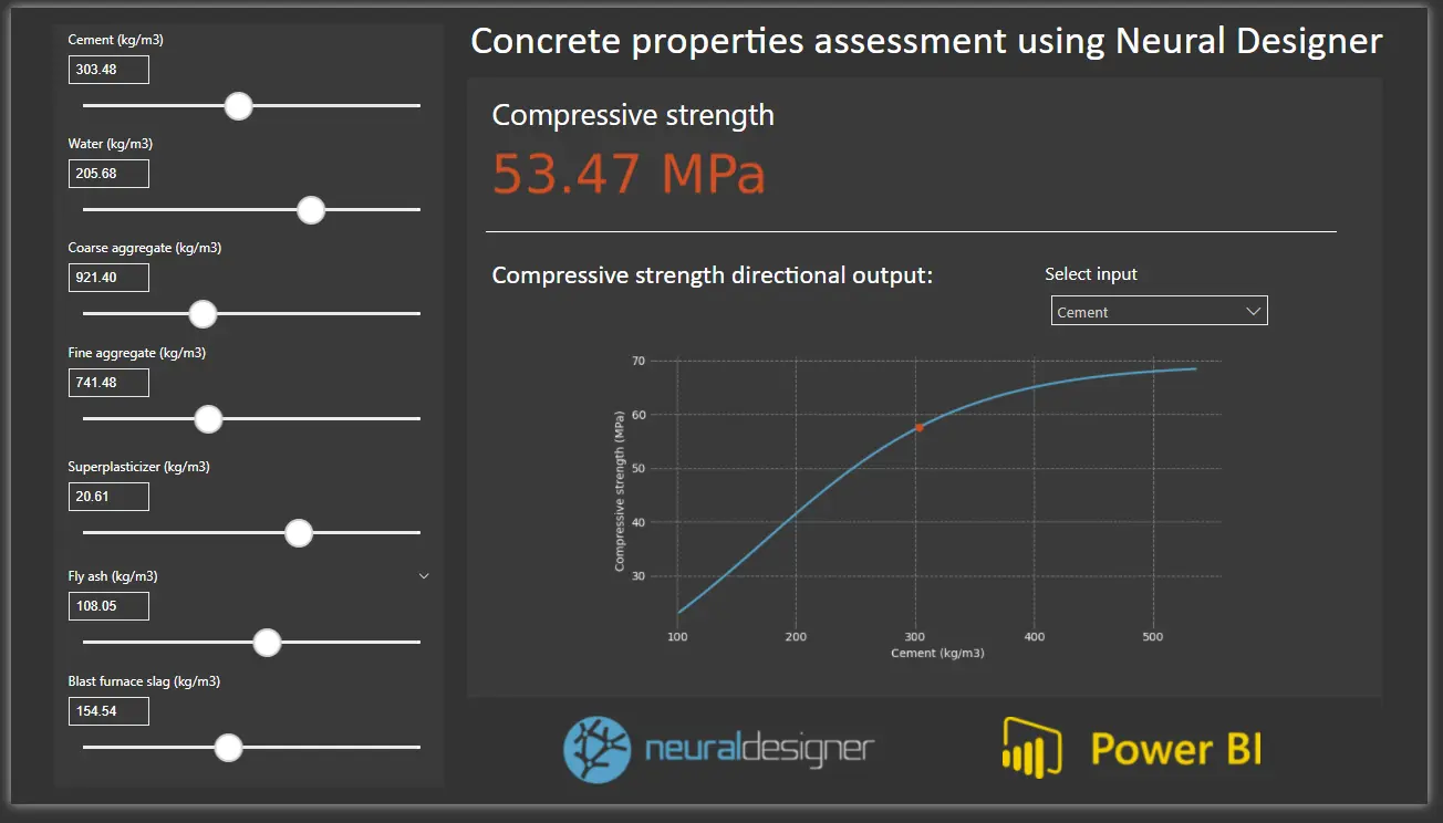
We can give the report the format we desire, and use it for a formal presentation or as a powerful Bussiness Intelligence tool.

To learn more, see the next example:

Related posts